Why?
Two Reasons:
1. Eigenfaces is probably one of the simplest face recognition methods and also rather old, then why worry about it at all? Because, while it is simple it works quite well. And it’s simplicity also makes it a good way to understand how face recognition/dimensionality reduction etc works.
2. I was thinking of writing a post based on face recognition in Bees next, so this should serve as a basis for the next post too. The idea of this post is to give a simple introduction to the topic with an emphasis on building intuition. For more rigorous treatments, look at the references.
_____
Introduction
Like almost everything associated with the Human body – The Brain, perceptive abilities, cognition and consciousness, face recognition in humans is a wonder. We are not yet even close to an understanding of how we manage to do it. What is known is that it is that the Temporal Lobe in the brain is partly responsible for this ability. Damage to the temporal lobe can result in the condition in which the concerned person can lose the ability to recognize faces. This specific condition where an otherwise normal person who suffered some damage to a specific region in the temporal lobe loses the ability to recognize faces is called prosopagnosia. It is a very interesting condition as the perception of faces remains normal (vision pathways and perception is fine) and the person can recognize people by their voice but not by faces. In one of my previous posts, which had links to a series of lectures by Dr Vilayanur Ramachandran, I did link to one lecture by him in which he talks in detail about this condition. All this aside, not much is known how the perceptual information for a face is coded in the brain too.

_____
A Motivating Parallel
Eigenfaces has a parallel to one of the most fundamental ideas in mathematics and signal processing – The Fourier Series. This parallel is also very helpful to build an intuition to what Eigenfaces (or PCA) sort of does and hence must be exploited. Hence we review the Fourier Series in a few sentences.
Fourier series are named so in the honor of Jean Baptiste Joseph Fourier (Generally Fourier is pronounced as “fore-yay”, however the correct French pronunciation is “foor-yay”) who made important contributions to their development. Representation of a signal in the form of a linear combination of complex sinusoids is called the Fourier Series. What this means is that you can’t just split a periodic signal into simple sines and cosines, but you can also approximately reconstruct that signal given you have information how the sines and cosines that make it up are stacked.
More Formally: Put in more formal terms, suppose  is a periodic function with period
  defined in the interval
  and satisfies a set of conditions called the Dirichlet’s conditions:
1.  is finite, single valued and its integral exists in the interval.
2. has a finite number of discontinuities in the interval.
3. has a finite number of extrema in that interval.
then can be represented by the trigonometric series
![f(x) = \displaystyle\frac{a_0}{2} + \displaystyle \sum_{n=1}^\infty [a_n cos(nx) + b_n sin(nx) ]\qquad(1)](https://s0.wp.com/latex.php?latex=f%28x%29+%3D+%5Cdisplaystyle%5Cfrac%7Ba_0%7D%7B2%7D+%2B+%5Cdisplaystyle+%5Csum_%7Bn%3D1%7D%5E%5Cinfty+%5Ba_n+cos%28nx%29+%2B+b_n+sin%28nx%29+%5D%5Cqquad%281%29&bg=ffffff&fg=333333&s=0&c=20201002)
The above representation of is called the Fourier series and the coefficients  ,
,  and
and  are called the fourier coefficients and are determined from by Euler’s formulae. The coefficients are given as :
Note: It is common to define the above using 
An example that illustrates  or the Fourier series is:
 [Image Source]
A square wave (given in black) can be approximated to by using a series of sines and cosines (result of this summation shown in blue). Clearly in the limiting case, we could reconstruct the square wave exactly with simply sines and cosines.
_____
Though not exactly the same, the idea behind Eigenfaces is similar. The aim is to represent a face as a linear combination of a set of basis images (in the Fourier Series the bases were simply sines and cosines). That is :

Where  represents the
  face with the mean subtracted from it,
  represent weights and
  the eigenvectors. If this makes somewhat sketchy sense then don’t worry. This was just like mentioning at the start what we have to do.
The big idea is that you want to find a set of images (called Eigenfaces, which are nothing but Eigenvectors of the training data) that if you weigh and add together should give you back a image that you are interested in (adding images together should give you back an image, Right?). The way you weight these basis images (i.e the weight vector) could be used as a sort of a code for that image-of-interest and could be used as features for recognition.
This can be represented aptly in a figure as:

Click to Enlarge
In the above figure, a face that was in the training database was reconstructed by taking a weighted summation of all the basis faces and then adding to them the mean face. Please note that in the figure the ghost like basis images (also called as Eigenfaces, we’ll see why they are called so) are not in order of their importance. They have just been picked randomly from a pool of 70 by me. These Eigenfaces were prepared using images from the MIT-CBCL database (also I have adjusted the brightness of the Eigenfaces to make them clearer after obtaining them, therefore the brightness of the reconstructed image looks different than those of the basis images).
_____
An Information Theory Approach:
First of all the idea of Eigenfaces considers face recognition as a 2-D recognition problem, this is based on the assumption that at the time of recognition, faces will be mostly upright and frontal. Because of this, detailed 3-D information about the face is not needed. This reduces complexity by a significant bit.
Before the method for face recognition using Eigenfaces was introduced, most of the face recognition literature dealt with local and intuitive features, such as distance between eyes, ears and similar other features. This wasn’t very effective. Eigenfaces inspired by a method used in an earlier paper was a significant departure from the idea of using only intuitive features. It uses an Information Theory appraoch wherein the most relevant face information is encoded in a group of faces that will best distinguish the faces. It transforms the face images in to a set of basis faces, which essentially are the principal components of the face images.
The Principal Components (or Eigenvectors) basically seek directions in which it is more efficient to represent the data. This is particularly useful for reducing the computational effort. To understand this, suppose we get 60 such directions, out of these about 40 might be insignificant and only 20 might represent the variation in data significantly, so for calculations it would work quite well to only use the 20 and leave out the rest. This is illustrated by this figure:

Click to Enlarge
Such an information theory approach will encode not only the local features but also the global features. Such features may or may not be intuitively understandable. When we find the principal components or the Eigenvectors of the image set, each Eigenvector has some contribution from EACH face used in the training set. So the Eigenvectors also have a face like appearance. These look ghost like and are ghost images or Eigenfaces. Every image in the training set can be represented as a weighted linear combination of these basis faces.
The number of Eigenfaces that we would obtain therefore would be equal to the number of images in the training set. Let us take this number to be  . Like I mentioned one paragraph before, some of these Eigenfaces are more important in encoding the variation in face images, thus we could also approximate faces using only the
  most significant Eigenfaces.
_____
Assumptions:
1. There are images in the training set.
2. There are most significant Eigenfaces using which we can satisfactorily approximate a face. Needless to say K < M.
3. All images are  matrices, which can be represented as
  dimensional vectors. The same logic would apply to images that are not of equal length and breadths. To take an example: An image of size 112 x 112 can be represented as a vector of dimension 12544 or simply as a point in a 12544 dimensional space.
_____
Algorithm for Finding Eigenfaces:
1. Obtain training images  ,
,  …
…  , it is very important that the images are centered.

2. Represent each image  as a vector
  as discussed above.

Note: Due to a recent WordPress  bug, there is some trouble with constructing matrices with multiple columns. To avoid confusion and to maintain continuity, for the time being I am posting an image for the above formula that’s showing an error message. Same goes for some formulae below in the post.
 3. Find the average face vector
  .
.

4. Subtract the mean face from each face vector to get a set of vectors  . The purpose of subtracting the mean image from each image vector is to be left with only the distinguishing features from each face and “removing” in a way information that is common.

5. Find the Covariance matrix  :
:
 , where
 ![A=[\Phi_1, \Phi_2 \ldots \Phi_M]](https://s0.wp.com/latex.php?latex=A%3D%5B%5CPhi_1%2C+%5CPhi_2+%5Cldots+%5CPhi_M%5D&bg=ffffff&fg=333333&s=0&c=20201002)
Note that the Covariance matrix has simply been made by putting one modified image vector obtained in one column each.
Also note that is a  matrix and
  is a
is a  matrix.
6. We now need to calculate the Eigenvectors  of , However note that is a matrix and it would return
  Eigenvectors each being dimensional. For an image this number is HUGE. The computations required would easily make your system run out of memory. How do we get around this problem?
7. Instead of the Matrix  consider the matrix
  . Remember is a matrix, thus is a
  matrix. If we find the Eigenvectors of this matrix, it would return Eigenvectors, each of Dimension
  , let’s call these Eigenvectors
  .
.
Now from some properties of matrices, it follows that:  . We have found out earlier. This implies that using we can calculate the M largest Eigenvectors of . Remember that
  as M is simply the number of training images.
8. Find the best Eigenvectors of  by using the relation discussed above. That is: . Also keep in mind that
  .
.

[6 Eigenfaces for the training set chosen from the MIT-CBCL database, these are not in any order]
9. Select the best Eigenvectors, the selection of these Eigenvectors is done heuristically.
_____
Finding Weights:
The Eigenvectors found at the end of the previous section, when converted to a matrix in a process that is reverse to that in STEP 2, have a face like appearance. Since these are Eigenvectors and have a face like appearance, they are called Eigenfaces. Sometimes, they are also called as Ghost Images because of their weird appearance.
Now each face in the training set (minus the mean), can be represented as a linear combination of these Eigenvectors :
 m, where ‘s are Eigenfaces.
These weights can be calculated as :
 .
.
Each normalized training image is represented in this basis as a vector.

 where i = 1,2… M. This means we have to calculate such a vector corresponding to every image in the training set and store them as templates.
_____
Recognition Task:
Now consider we have found out the Eigenfaces for the training images , their associated weights after selecting a set of most relevant Eigenfaces and have stored these vectors corresponding to each training image.
If an unknown probe face  is to be recognized then:
1. We normalize the incoming probe as  .
.
2. We then project this normalized probe onto the Eigenspace (the collection of Eigenvectors/faces) and find out the weights.
 .
.
3. The normalized probe  can then simply be represented as:


After the feature vector (weight vector) for the probe has been found out, we simply need to classify it. For the classification task we could simply use some distance measures or use some classifier like Support Vector Machines (something that I would cover in an upcoming post). In case we use distance measures, classification is done as:
Find 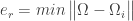 . This means we take the weight vector of the probe we have just found out and find its distance with the weight vectors associated with each of the training image.
And if  , where
  is a threshold chosen heuristically, then we can say that the probe image is recognized as the image with which it gives the lowest score.
If however  then the probe does not belong to the database. I will come to the point on how the threshold should be chosen.
For distance measures the most commonly used measure is the Euclidean Distance. The other being the Mahalanobis Distance. The Mahalanobis distance generally gives superior performance. Let’s take a brief digression and look at these two simple distance measures and then return to the task of choosing a threshold.
_____
Distance Measures:
Euclidean Distance: The Euclidean Distance is probably the most widely used distance metric. It is a special case of a general class of norms and is given as:

The Mahalanobis Distance: The Mahalanobis Distance is a better distance measure when it comes to pattern recognition problems. It takes into account the covariance between the variables and hence removes the problems related to scale and correlation that are inherent with the Euclidean Distance. It is given as:

Where is the covariance between the variables involved.
_____
Deciding on the Threshold:
Why is the threshold, important?
Consider for simplicity we have ONLY 5 images in the training set. And a probe that is not in the training set comes up for the recognition task. The score for each of the 5 images will be found out with the incoming probe. And even if an image of the probe is not in the database, it will still say the probe is recognized as the training image with which its score is the lowest. Clearly this is an anomaly that we need to look at. It is for this purpose that we decide the threshold. The threshold is decided heuristically.

Click to Enlarge
Now to illustrate what I just said, consider a simpson image as a non-face image, this image will be scored with each of the training images. Let’s say  is the lowest score out of all. But the probe image is clearly not beloning to the database. To choose the threshold we choose a large set of random images (both face and non-face), we then calculate the scores for images of people in the database and also for this random set and set the threshold (which I have mentioned in the “recognition” part above) accordingly.
_____
More on the Face Space:
To conclude this post, here is a brief discussion on the face space.
 [Image Source – [1]]
Consider a simplified representation of the face space as shown in the figure above. The images of a face, and in particular the faces in the training set should lie near the face space. Which in general describes images that are face like.
The projection distance  should be under a threshold as already seen. The images of known individual fall near some face class in the face space.
There are four possible combinations on where an input image can lie:
1. Near a face class and near the face space : This is the case when the probe is nothing but the facial image of a known individual (known = image of this person is already in the database).
2. Near face space but away from face class : This is the case when the probe image is of a person (i.e a facial image), but does not belong to anybody in the database i.e away from any face class.
3. Distant from face space and near face class : This happens when the probe image is not of a face however it still resembles a particular face class stored in the database.
4. Distant from both the face space and face class: When the probe is not a face image i.e is away from the face space and is nothing like any face class stored.
Out of the four, type 3 is responsible for most false positives. To avoid them, face detection is recommended to be a part of such a system.
_____
References and Important Papers
1.Face Recognition Using Eigenfaces, Matthew A. Turk and Alex P. Pentland, MIT Vision and Modeling Lab, CVPR ’91.
2. Eigenfaces Versus Fischerfaces : Recognition using Class Specific Linear Projection, Belhumeur, Hespanha, Kreigman, PAMI ’97.
3. Eigenfaces for Recognition, Matthew A. Turk and Alex P. Pentland, Journal of Cognitive Neuroscience ’91.
_____
Related Posts:
1. Face Recognition/Authentication using Support Vector Machines
2. Why are Support Vector Machines called so
_____
MATLAB Codes:
I suppose the MATLAB codes for the above are available on atleast 2-3 locations around the internet.
However it might be useful to put out some starter code. Note that the variables have the same names as those in the description above.You may use this mat file for testing. These are the labels for that mat file.
%This is the starter code for only the part for finding eigenfaces.

load('features_faces.mat'); % load the file that has the images.
%In this case load the .mat filed attached above.
% use reshape command to see an image which is stored as a row in the above.

% The code is only skeletal.
% Find psi - mean image
Psi_train = mean(features_faces')';
% Find Phi - modified representation of training images.
% 548 is the total number of training images.
for i = 1:548
    Phi(:,i) = raw_features(:,i) - Psi_train;
end
% Create a matrix from all modified vector images
A = Phi;
% Find covariance matrix using trick above
C = A'*A;
[eig_mat, eig_vals] = eig(C);
% Sort eigen vals to get order
eig_vals_vect = diag(eig_vals);
[sorted_eig_vals, eig_indices] = sort(eig_vals_vect,'descend');
sorted_eig_mat = zeros(548);
for i=1:548
    sorted_eig_mat(:,i) = eig_mat(:,eig_indices(i));
end
% Find out Eigen faces
Eig_faces = (A*sorted_eig_mat);
size_Eig_faces=size(Eig_faces);
% Display an eigenface using the reshape command.

% Find out weights for all eigenfaces
% Each column contains weight for corresponding image
W_train = Eig_faces'*Phi;
face_fts = W_train(1:250,:)'; % features using 250 eigenfaces.

_____
Onionesque Reality Home >>
					Read Full Post »


 , where
  represents the features and
  the class label, that could be either 1 or -1. On training we obtain a set of Support Vectors
  , multipliers
  ,
,  and the term
  . To understand what
  in the equation of a straight line,
  . The terms
  and
and  determine the orientation of the
 are the support vectors.


 to:
to:
 , the identity is accepted if:


 class problem. Where
 having
  training images belonging to
  ofcourse. It is from
  that we generate the two classes I mentioned above.
 and
and  are images and
  indicates that they belong to the same person.
 indicates that they do not belong to the same person.
 is presented.
 or else reject it. I have discussed the need for a threshold


