This post is part of a series on face recognition, I have been posting on face recognition for a while. There would be at least 7-8 more posts in the near future on the topic. Though I can not promise a time frame within which all would be up.
Previous Related Posts:
1. Face Recognition using Eigenfaces and Distance Classifiers – A Tutorial
3. A Huge Collection of Datasets (Post links to a number of face image databases)
4. Why are Support Vector Machines called so?
This post would reference two of my posts. One on SVMs and the other on Face Recognition using Eigenfaces.
Note: This post focuses on the idea behind using SVMs for face recognition and authentication. In future posts I will cover the various packages that can be used to implement SVMs and how to go about using them, and specifically for face recognition. The same can be easily extended to other similar problems such as content based retrieval systems, speech recognition, character or signature verification systems as well.
_____
Difference between Face Authentication (Verification) and Face Recognition (also called identification):
This might seem like a silly thing to start with. But for the sake of completeness, It is a good point to start with.
Face Authentication can be considered a subset of face recognition. Though due to the small difference there are a few non-concurrent parts in both the systems.
Face Authentication (also called verification) involves a one to one check that compares an input image (also called a query image, probe image or simply probe) with only the image (or class) that the user claims to be. In simple words, if you stand in front of a face authentication system and claim to be a certain user, the system will ONLY check if you are that user or not.

Face Recognition (or Identification) is another thing, though ofcourse related. It involves a one to many comparison of the input image (or probe or query image) with a template library. In simple words, in a face recognition system the input image will be compared with ALL the classes and then a decision will be made so as to identify to WHO the the input image belongs to. Or if it does not belong to the database at all.

Like I just said before, though both Authentication and Recognition are related there are some differences in the method involved, which are obvious due to the different nature of both.
_____
A Touch-Up of Support Vector Machines:
A few posts ago I wrote a post on why Support Vector Machines had this rather “seemingly” un-intuitive name. It had a brief introduction to SVMs as well. For those completely new to Support Vector Machines this post should help. I’ll still add a little for this post.
Support Vector Machine is a binary classification method that finds the optimal linear decision surface between two classes. The decision surface is nothing but a weighted combination of the support vectors. In other words, the support vectors decide the nature of the boundary between the two classes. Take a look at the image below:

The SVM takes in labeled training examples 


As is indicated in the diagram, the linear decision surface is :

where
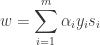
where 
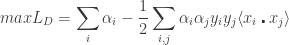
The above holds when the data (classes) is linearly separable. Sometimes however, that’s not the case. Take the following example:
The two classes are indicated by the two different colors. The data is clearly not LINEARLY separable.

However when mapped onto two dimensions, a linear decision surface between them can be made with ease.
 Take another example. In this example the data is not linearly separable in 2-D, so they are mapped onto three dimensions where a linear decision surface between the classes can be made.

By Cover’s Theorem it is more likely that a data-set not linearly separable in some dimension would be linearly separable in a higher dimension. The above two examples are simple, sometimes the data might be linearly separable at very high dimensions, maybe at infinite dimensions.
But how do we realize it? This done by employing the beautiful Kernel Trick. In place of the inner products we use a suitable Mercer Kernel. I don’t believe it is a good idea to discuss kernels here, or it will be a needless digression from face recognition. I promise to discuss it some time later.
Thus the non-linear decision surface changes from 

Where 
_____
Face Authentication is a two class problem. As I have mentioned earlier, here the system is presented with a claimed identity and it has to make a decision whether the claimant is really that person or not. The SVM in such applications will have to be fed with the images of one person, which will constitute one class and the other class will consist of images of other people other than that person. The SVM will then generate a linear decision surface.
For a input/probe image 

Or it is rejected. We can parameterize the decision surface by modifying the above as:

Then, a claim will be accepted if for a probe,

_____
Now face recognition is a 
Feature Extraction: The faces will have to be represented by some appropriate features, these could be weights obtained using the Eigenfaces method, or using gabor features or anything else. I have written a post earlier that talked of a face recognition system based on Eigenfaces. I would direct the reader to check face representation using Eigenfaces there.
Using Eigenfaces, each probe 

After obtaining such a weight vector for the input or probe image and for all the other images stored in the library, we were simply finding the Euclidean or the Mahalanobis distance of the weight vector of the probe image with those of the images in the template library. And then were recognizing the probe as a face that gave the minimum score provided it was below a certain threshold. I have discussed this is much detail there. And since I have, I would not discuss this again here.
_____
Representation in Difference Space:
SVMs are binary classifiers, that is – they give the class which might be 1 or -1, so we would have to modify the representation of faces a little bit than what we were doing in that previous post to make it somewhat more desirable. In the previous approach that is “a view based or face space approach”, each image was encoded separately. Here, we would change the representation and encode faces into a difference space. The difference space takes into account the dissimilarities between faces.
In the difference space there can be two different classes.
1. The class that encodes the dissimilarities between different images of the same person,
2. The other class encodes the dissimilarities between images of other people. These two classes are then given to a SVM which then generates a decision surface.
As I wrote earlier, Face recognition traditionally can be thought of as a
Now consider a training set 


1. The within class differences set. This set takes into account the differences in the images of the same class or individual. In more formal terms:

Where 


This set contains the differences not just for one individual but for all
2. The between class differences set. This set gives the dissimilarities of different images of different individually. In more formal terms:

Where 
_____
Face Authentication:
For Authentication the incoming probe 
Using this, we first find out the similarity score:

We then accept this claim if it lies below a certain threshold 
_____
Face Recognition:
Consider a set of images
We take

The image with the lowest score but below a threshold is recognized. I have written at the end of this post explaining why this threshold is important. This threshold is mostly chose heuristically.
_____
References and Important Papers
1. Face Recognition Using Eigenfaces, Matthew A. Turk and Alex P. Pentland, MIT Vision and Modeling Lab, CVPR ‘91.
2. Eigenfaces Versus Fischerfaces : Recognition using Class Specific Linear Projection, Belhumeur, Hespanha, Kreigman, PAMI ‘97.
3. Eigenfaces for Recognition, Matthew A. Turk and Alex P. Pentland, Journal of Cognitive Neuroscience ‘91.
4. Support Vector Machines Applied to Face Recognition, P. J. Phillips, Neural Information Processing Systems ’99.
5. The Nature of Statistical Learning Theory (Book), Vladimir Vapnik, Springer ’99.
6. A Tutorial on Support Vector Machines for Pattern Recognition, Christopher J. C. Burges, Data Mining and Knowledge Discovery, ’99
_____
 .
.

 dimensional space.
 w.r.t a specific training example
  is defined as:
 , for a large functional margin (greater confidence in correct prediction) we want
 , for a large functional margin we want
 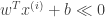 .
.
 ,
, 
 and
and  .
.
 ,
,
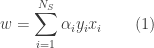
 is the number of support vectors and the
  s represent the Lagrangian multipliers.
 and suppose the
  support vector exerts a force of
  on a stiff sheet lying along the decision surface.
  represents the unit vector in the direction
  then satisfies the conditions for mechanical equilibrium:
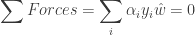
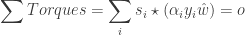
 denotes the vector product.


