Blind Geometers

This post is of general interest.

I was reading Prof. Alexei Sossinsky ‘s coffee table book on Knots – Knots: Mathematics with a Twist*, and it mentioned a couple of interesting cases of blind mathematicians. These couple of cases ignited enough interest to publish an old draft on blind mathematicians albeit now with a different flavor.

*(Note that the book has poor reviews on Amazon which I honestly don’t relate to. I think the errors reported in the reviews have been corrected plus the book is extremely short ~ 100 pages and hence actually readable on a few coffee breaks)

Sossinsky’s book gives an example of Antoine’s Necklace:

Antoine’s Necklace: A Wild Knot

Antoine’s Necklace is a Wild Knot that can be constructed as follows:

1. Start with a solid torus say .

2. Place inside it four smaller tori linked two by two to make a chain. Let’s call this chain .

3.  Inside each of the tori in step 2, construct a similar chain. This would be a set of 16 tori. Let’s call this

4. Repeat this process ad-infinitum. The set obtained by the infinite set of Tori will be Antoine’s necklace.

Antoine’s Necklace is not a mere curiosity and has very interesting properties. One would suppose that constructing such a structure would require considerable visualization, which is indeed true. However one of the most interesting things about this knot is that it was formulated and studied by Louis Antoine, who was blind. After he lost his eyesight, the famous mathematician Henri Lebesgue suggested to him that he study topology.

_______________

I have noticed (it is a common observation) that it is almost a rule that mathematicians who are blind are usually geometers/topologists. Such a correlation can not be mere coincidence.

Before reading Sossinsky’s book which also mentions G. Ya. Zuev as another influential blind topologist, the two best examples that I was aware of were L. S. Pontryagin and the great Leonhard Euler. Pontryagin is perhaps the first blind mathematician that I had heard of who made seminal contributions to numerous areas of mathematics (Algebraic Topology, Control Theory and Optimization to name a few). Some of his contributions are very abstract while some such as those in control theory are also covered in advanced undergrad textbooks (that is how I heard of him).

Lev Pontryagin (1908-1988)

Pontryagin lost his eyesight at the age of 14 and thus made all of his illustrious contributions (and learnt most of his mathematics) while blind. The case was a little different for Euler. He learnt most of his earlier mathematics while not blind. Born in 1707, he almost lost eyesight in the right eye in 1735. After that his eyesight worsened, losing it completely in 1766 to cataract.

Euler (1707-1783) on a Swiss Banknote

His mathematical productivity however actually increased, publishing more than half of his work after losing eyesight. Remarkably he published one paper each week in 1775 aided by students who doubled up as scribes. It is noteworthy that he is the most prolific mathematician to have ever lived in terms of number of pages published (Paul Erdős produced more papers), becoming one of the most influential mathematicians to have ever lived.

_______________

This excellent (as usual) Notices of the AMS article lists a few more famous blind mathematicians. Bernard Morin and Nicholas Suanderson to name a couple. Bernard Morin is famous for his work on sphere eversion (i.r homotopy, many youtube videos on this theme are available, video below).

Morin’s Surface

It is difficult to imagine for ordinary people that such work could be done by somebody who has been blind since age six. What could be the explanation for what I atleast consider an extraordinary and counter intuitive case?

Sossinsky in his book talks briefly of what he thinks about it and of some research in the area (though he doesn’t point out specific papers, it turns out there is a lot of interesting work on this aspect on spatial representation in blind people). He writes:

“It is not surprising at all that almost all blind mathematicians are geometers. The spatial intuition that sighted people have is based on the image of the world that is projected on their retinas; thus it is a two (and not three) dimensional image that is analysed in the brain of a sighted person. A blind person’s spatial intuition on the other hand, is primarily the result of tile and operational experience. It is also deeper – in the literal as well as the metaphorical sense. […]

recent biomathematical studies have shown that the deepest mathematical structures, such as topological structures, are innate, whereas finer structures, such as linear structures are acquired. Thus, at first, the blind person who regains his sight does not distinguish a square from a circle: He only sees their topological equivalence. In contrast, he immediately sees that a torus is not a sphere […]”

The Notices article has a line: “In such a study the eyes of the spirit and the habit of concentration will replace the lost vision”, referring to what is called as the Mind’s Eye commonly (i.e it is commonly believed that people with disabilities have some other senses magnified). Some of the work of the celebrated neuroscientist Oliver Sacks  (who I also consider as one of my role models. Movie buffs would recognize him from Dr Malcolm Sayer’s character in the fantastic movie Awakenings) talks of individuals in which this was indeed the case. He documents some of such cases in his book, The Mind’s Eye. He also notes that such magnification ofcourse does not happen in all of his patients but only in some fascinating cases.

The Mind’s Eye by Oliver Sacks (Click on image to view on Amazon)

Here in the video below (many more available on youtube) Dr Sacks describes some of such cases:

I wonder when we’d know enough. For such cases tell us something interesting about the brain, it’s adaptability, vision and spatial representation.

The Notices article also cites some examples of famous blind mathematicians who were not geometers, perhaps the more interesting cases if I could loosely put it that way.

_______________

Translation of the Article in Romanian:

Geometri Blind by Alexander Ovsov

Recommendations

1. The World of Blind Mathematicians – Notices of the AMS, Nov 2002  (pdf)

2. The Mind’s Eye – Oliver Sacks (Amazon)

3. Knots Mathematics with a Twist – Alexiei Sossinsky (Amazon)

4. Biography of Lev Pontryagin

5. Mathematical Reasoning and External Symbolic Systems – Catarina Dulith Novaes

_______________

Onionesque Reality Home >>

Read Full Post »

Blind Source Separation in Magnetic Resonance Images

I have been involved in a major project on contrast enhancement of Magnetic Resonance Images by using Independent Component Analysis (ICA) and Support Vector Machines (SVM) for the past couple of  months. It is an extremely exciting project and also something new for me, as I have worked on bio-medical images just once before. In the past, I have used ICA and SVM in face recognition/authentication, however this application is quite novel.

This post intends to introduce the problem, discuss a motivating example, some methods, expected work and some problems.

__________

A Simple Introduction and Motivating Example:

The simplest motivating example for this problem is the famous cocktail party problem:

You are at a cocktail party, and there are about 12 people present with each talking simultaneously. Add to that a music source. So that makes it 13.

Suppose you want to follow what each person was saying later and for doing so you place a number of tape recorders at different locations in the room (let’s not worry about the number of recorders right now). When you hear them later, the sounds would hardly be understandable as they would be mixed up.

Now you define an engineering problem : that using these recordings (which are basically mixtures), separate out the different sources with as little distortion as possible. In a real time cocktail party, the brain shows^[1][2][3] a remarkable ability to follow one conversation. However such a problem has proved to be quite difficult in signal processing. Let’s just illustrate the cocktail party problem in a cartoon below :

 

The Cocktail Party Problem

Please listen to a demo of the cocktail party problem at the HUT ICA project page.

__________

The Logic Behind Constructing MR Images in Simple Terms:

Now, keeping the previous brief discussion in mind. Let’s introduce in simple words how MRI works. This is just a simplification to make the idea clearer, and not really how MRI works.  Discussing MRI in detail would divert the focus of the post. To look at how MRI works follow these highly recommended tutorials^[4][5][6]:

Suppose your body is placed in a Magnetic Field (let’s not worry about specifics yet). Consider two contiguous tissues in your body – X and Y. When subject to a magnetic field, the particles (protons) in the tissues would get aligned according to the field. The amount of magnetization would depend on the tissue type. Now suppose we want to measure how much a tissue gets magnetized. One way to think about it is like this : First apply the magnetic field, after the application the particles would get excited. Once the field is removed, these particles would tend to relax to their ground state. By being able to measure the time it takes for the particles to return, we would get some measure of the magnetization of the tissue(s). This is because, the greater the time for relaxation, greater the magnetization.

An image is basically a measure of the energy distribution. Now suppose we have the measurements for tissues X and Y, and since they were of a different nature (composition, density of protons etc), their response to the field would have been different. Thus we would get some contrast between them and thus would get an image.

In very simplistic terms, this is how MRI scans are obtained. Though as mentioned above, please follow [4][5][6] for detailed tutorials on MRI.

__________

MRI scans of the Brain and the Cocktail Party Problem :

Now consider the above discussion in context of taking a MRI scan of the brain. The brain has a number of constituents. Some being : Gray Matter, White Matter, Cerebrospinal Fluid (CSF) Fat, Muscle/Skin, Glial Matter etc. Now since each is unique, they would exhibit unique characteristics under a magnetic field. However, while taking a scan, we get one MRI image of the entire brain.

These scans can be considered as an equivalent to the mixtures of the cocktail party example. If we apply blind source separation to these, we should be able to separate out the various constituents such as gray matter, white matter, CSF etc. These images of the independent sources can be used for better diagnosis. This would be something like this :

If suppose the Simulated MR scans (from the McGill Simulated brain Database) were as follows:

 

Simulated MR Scans

 

 

The “ground truth” images for these scans would be as follows :

 

Ground Truth Images of Different Brain Tissue Substances

__________

Restatement of the Broad Research Problem and Use of ICA and SVM:

Magnetic Resonance Imaging is superior to Computerised Tomography for brain imaging at least, for the reason that it can give much better soft tissue contrast (because even small changes in the proton density and composition in the tissue are well represented).

Like for most techniques, improvements to scans obtained by MRI are much desired to improve diagnosis. Blind source separation has been used to separate physiologically different components from EEG^[7]/MEG^[8] data (similar to the cocktail party problem), financial data^[9] and even in fMRI^[10][11]. But it has not received much attention for MRI. Nakai et al^[12] used Independent Component Analysis for the purpose of separating physiologically independent components from MRI scans. They took MR images of 10 normal subjects, 3 subjects with brain tumour and 1 subject with multiple sclerosis and performed ICA on the data. They reported success in improving contrast for gray and white matter, which was beneficial for the diagnosis of brain tumour. The demylination in Multiple sclerosis cases was also enhanced in the images. They suggested that ICA could potentially separate out all the tissues which had different relaxation characteristics (different sources of the cocktail party example). This approach thus shows much promise.

In more technical terms : Consider a set of MR frames as a single multispectral image. Where each band is taken during a particular pulse sequence (will be discussed below). Then use ICA on the data to separate out the physiologically independent components. A classifier such as the SVM can improve the contrast further of the separated independent components.

However, using ICA for MRI has been tricky, something I would discuss towards the end of this post and also in future posts.

Before doing so, I intend to touch up on the basics for the sake of completeness.

__________

Magnetic Resonance Imaging:

I had been thinking of writing a detailed tutorial on MRI, mostly because it requires some basic physics. However I don’t think it is required. I would recommend [4][5][6] for a study of the same in sufficient depth. I have recently taken tutorials on MRI, and would be willing to write for the blog if there are requests.

__________

An Introduction to Independent Component Analysis:

Independent Component Analysis was developed initially to solve problems such as the cocktail party problem discussed above.

Let’s formalize a problem like the cocktail party example. For simplicity let us assume that there are only two sources and two mixtures (obtained by keeping two recorders at different locations in the party).

Let’s represent these two mixtures as and , and let and be the two sources that were mixed. Since we are assuming that the two microphones were kept at different locations, the mixtures and would be different.

We could write this as:

The coefficients are basically some parameters that depend on the distance of the respective source from the microphones.

Let’s define our problem as : Using only the mixtures estimate the signal sources . It is notable that you do not have any knowledge of the parameters .

This could be illustrated by this :

Consider three signals:

Suppose we have five mixtures obtained from these three signals.

Signals obtained by mixing source signals

If you only have the mixed signals available. And do not know how they were mixed (parameters not known). And from these mixed signals () you have to estimate the source signals (). This problem is of considerable difficulty.

One approach would be : Use the statistical properties of the signals () to estimate the parameters (). It is surprising that it is enough to assume that and are statistically independent. This assumption might not be valid in many scenarios. But works well in most situations.

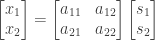
We could write the above system of linear equations in matrix form as :

where, represents the mixing matrix, and represent the mixtures and the sources respectively.

The problem is to estimate from without knowing . The assumption made is that the sources are statistically independent.

How we go about solving this problem is exciting and an area of active research.  ICA was originally developed for solving such problems. Please follow [12][13][14] for discussions on mutual information, measures of non-gaussianity such as Kurtosis and Negentropy and the fastICA algorithm.

__________

Why can ICA be used in MRI?

One limitation that ICA faces is that it can not work if more than one signal sources have a  Gaussian distribution. This can be illustrated as follows:

Again consider our equation for just two sources :

Our problem was : We have to estimate from without any knowledge of . We would first need to estimate the parameters from , assuming statistical independence of . And then we could find as :

, where , or the inverse of the estimated mixing matrix .

To understand how a solution would become impossible if both the sources had a Gaussian distribution, consider this :

Consider two independent components having the following uniform distributions:

The joint density of the two sources would then be uniform on a square. This follows from the fact that the joint density would be the product of the two marginal densities.

 

The joint distribution for Si

[ Image Source : Reference [12][13] ]

Now if and were mixed by a mixing matrix

The mixtures obtained are and . Now since the original sources had a joint distribution on a square, and they were transformed by using a mixing matrix, the joint distribution of the mixtures and will be a parallelogram. These mixtures are no longer independent.

 

Joint Distribution of the mixtures

[ Image Source : Reference [12][13] ]

Now consider the problem once again : We have to estimate the mixing matrix from the mixtures , and using this estimated we have to estimate the sources .

From the above joint distribution we have a way to estimate . The edges of the parallelogram are in a direction given by the columns of . This is an intuitive way of estimating the mixing matrix : obtain the joint distributions of the mixtures, estimate the columns of the mixing matrix by finding the directions of the edges of the parallelogram. This solution gives a good intuitive feel of a in-principle solution of the problem( however, it isn’t practical).

However, now instead of two independent sources having a uniform distribution consider two independent sources having a Gaussian distribution. The joint distribution would be :

 

Joint Distribution when both Independent sources are Gaussian

[ Image Source : Reference [12][13] ]

Now going by the above discussion, because of the nature of the above joint distribution, it is not possible to estimate the mixing matrix from it.

Thus ICA fails when one or more independent components have a a gaussian distribution.

Noise in MRI is non-gaussian^[16], therefore ICA is suited for MRI.

__________

Problems in Using ICA for MRI Blind Source Separation:

The application of ICA for MRI faces a number of problems. I would discuss these in later blog posts. I would only discuss one major problem – the problem of Over-Complete ICA.

Over-Complete ICA in MRI:

The problem of over complete ICA occurs when there are lesser sensors (tape recorders from our above discussion) than sources. This problem can be understood by the following discussion. Suppose you have 3 mixtures , and (imagine you have collected 3 tape recordings in a cocktail party of 6). Therefore you now have to estimate 6 sources from 3 mixtures.

Now the problem becomes something like this :

Assume for a second we can still estimate , still we can not find all the signal sources. As the number of linear equations is just three, while the number of unknowns is 6. This is a considerably harder problem and has been discussed by many groups such as [19][20][21].

Now dropping our assumption, the estimation of is also harder in such a case.

The Case in MRI:

The problem of over-complete ICA doesn’t arise when it comes to functional-MRI. However it is a problem when it comes to MRI^[17].

In MRI, by varying the parameters used for imaging, the three kind of images that can be obtained are T1 weighted, T2 weighted and Proton Density images. Going by our discussion in the section on MRI above. These three can be treated as mixtures.

Therefore, we have 3 mixtures at our disposal.  However, as the ground truth images above show: The number of different tissues in the brain exceeds 9. Thus this becomes a considerably difficult problem : We have to estimate 9-10 independent components from just 3 mixtures.

I would discuss methods that can help do that in later blog posts.

If only three mixtures are used, 3 ICs can be estimated. Since the actual number of ICs exceeds 9. It is obvious that the each of 3 ICs have atleast 2 ICs mixed, which means that a certain tissue type is not enhanced as much as it could have been had there been one IC for it. This can be understood by looking at this example.

 

3 ICs obtained by Applying Fast-ICA on MR scans

[I used FastICA for obtaining these Independent Components ]

To get more ICs, in simple words, we need more mixtures. However we can obtain more mixtures from the existing mixtures itself by a process of Band-Expansion^[18].

I would discuss this problem of OC-ICA and it’s possible solutions in later posts.

__________

To Conclude:

A basic idea related to application of ICA to MR scans was discussed. It is clear that even with just three ICs significant tissue contrast enhancement is achieved. Problems related to OC-ICA would be discussed in later posts one by one. I would also discuss quantifying the results obtained using the Tanimoto/Jaccard coefficient of similarity.

__________

References and Resources:

Cocktail Party Problem

[1] “Some Experiments on the Recognition of Speech, with One and with Two Ears“; E. Colin Cherry; The Journal of the Acoustical Society of America; September 1953. (PDF)

[2] “The Attentive Brain“; Stephen Grossberg; Department of Cognitive and Neural Systemss – Boston University; American Scientist, 1995. (PDF)

[3] “The Cocktail Party Problem : A Primer“; Josh H. McDermott; Current Biology Vol 19. No. 22. (PDF)

Magnetic Resonance Imaging

[4] “Magnetic Resonance ImagingTutorial“; H Panepucci and A Tannus; Technical Report; USP, 1994. (PDF)

[5] “10 Video lessons on MRI by Paul Callaghan” (~ an hour in total). (Videos)

[6] “MRI Tutorial for Neuroscience Boot Camp” Melissa Saenz. (PDF)

Sample ICA Applications Similar to The Cocktail Party Problem

[7] “Independent Component Analysis of Electroencephalographic Data“; Makieng, Bell, Jung, Sejnowski; Advances in Neural Information Processing Systems, 1996. (PDF)

[8] “Application of ICA to MEG noise Reduction“; Masaki Kawakatsu; 4th International Symposium on Independent Component Analysis and Blind Source Separation; 2003. (PDF)

[9] “Independent Component Analysis in Financial Data” from the book Computational Finance; Yasser S. Abu-Mostafa; The MIT Press; 2000. (Book Link)

[10] “ICA of functional MRI data : An overview“; Calhoun, Adali, Hansen, Larsen, Pekar; 4th International Symposium on Independent Component Analysis and Blind Source Separation; 2003. (PDF)

[11] “Independent Component Analysis of fMRI Data – Examining the Assumptions“; McKeown, Sejnowski; Human Brain Mapping; 1998. (PDF)

Independent Component Analysis : Tutorials/Books

[12] “Independent Component Analysis : Algorithms and Applications“; Aapo Hyvärinen, Erkki Oja; Neural Networks; 2000. (PDF)

[13] “Independent Component Analysis“; Aapo Hyvärinen, Juha Karhunen, Erkki Oja; John Wiley Publications; 2001. (Book Link)

[14] ICA Tutorial at videolectures.net by Aapo Hyvärinen. (Videos)

Independent Component Analysis for Magnetic Resonance Imaging

[15] “Application of of Independent Component Analysis to Magnetic Resonance Imaging for enhancing the Contrast of Gray and White Matter“; Nakai, Muraki, Bagarinao, Miki, Takehara, Matsuo, Kato, Sakahara, Isoda; NeuroImage; 2004. (Journal Link)

[16] “Noise in MRI“; Albert Macovski; Magnetic Resonance in Medicine; 1996. (PDF)

[17] “Independent Component Analysis in Magnetic Resonance Image Analysis“;  Ouyang, Chen, Chai, Clayton Chen, Poon, Yang, Lee; EURASIP journal on Advances in Signal Processing; 2008 (Journal Link)

[18] “Band Expansion Based Over-Complete Independent Component Analysis for Multispectral Processing of Magnetic Resonance Images “; Ouyang, Chen, Chai, Clayton Chen, Poon, Yang, Lee; IEEE Transactions on Biomedical Imaging; June 2008. (PDF)

Over-Complete ICA:

[19] “Blind Source Separation of More Sources Than Mixtures Using Over Complete Representations“; Lee, Lewicki, Girolami, Sejnowski; IEEE Signal Processing Letters; 1999. (PDF)

[20] “Learning Overcomplete Representations“; Lewicki, Sejnowski. (PDF)

[21] “A Fast Algorithm for estimating over-complete ICA bases for Image Windows “; Hyvarinen, Cristescu, Oja; International Joint Conference on Neural Networks; 1999. (IEEE Xplore link)

__________

Onionesque Reality Home >>

Read Full Post »

Some Interesting Courses: Neural Nets, Visualization, ML and Astrophysical Chemistry

Here are a number of interesting courses, two of which I am looking at for the past two weeks and that i would hopefully finish by the end of August-September.

Introduction to Neural Networks (MIT):

These days, amongst the other things that I have at hand including a project on content based image retrieval. I have been making it a point to look at a MIT course on Neural Networks. And needless to say, I am getting to learn loads.

I would like to emphasize that though I have implemented a signature verification system using Neural Nets, I am by no means good with them. I can be classified a beginner. The tool that I am more comfortable with are Support Vector Machines.

I have been wanting to know more about them for some years now, but I never really got the time or you can say the opportunity. Now that I can invest some time, I am glad I came across this course. So far I have been able to look at 7 lectures and I should say that I am MORE than very happy with the course. I think it is very detailed and extremely well suited for the beginner as well as the expert.

The instructor is H. Sebastian Seung who is the professor of computational neuroscience at the MIT.

The course has 25 lectures each one packed with a great amount of information. Meaning, the lectures might work slow for those who are not very familiar with this stuff.

The video lectures can be accessed over here. I must admit that i am a little disappointed that these lectures are not available on you-tube. That’s because the downloads are rather large in size. But I found them worth it any way.

The lectures cover the following:

Lecture 1: Classical neurodynamics
Lecture 2: Linear threshold neuron
Lecture 3: Multilayer perceptrons
Lecture 4: Convolutional networks and vision
Lecture 5: Amplification and attenuation
Lecture 6: Lateral inhibition in the retina
Lecture 7: Linear recurrent networks
Lecture 8: Nonlinear global inhibition
Lecture 9: Permitted and forbidden sets
Lecture 10: Lateral excitation and inhibition
Lecture 11: Objectives and optimization
Lecture 12: Excitatory-inhibitory networks
Lecture 13: Associative memory I
Lecture 14: Associative memory II
Lecture 15: Vector quantization and competitive learning
Lecture 16: Principal component analysis
Lecture 17: Models of neural development
Lecture 18: Independent component analysis
Lecture 19: Nonnegative matrix factorization. Delta rule.
Lecture 20: Backpropagation I
Lecture 21: Backpropagation II
Lecture 22: Contrastive Hebbian learning
Lecture 23: Reinforcement Learning I
Lecture 24: Reinforcement Learning II
Lecture 25: Review session

The good thing is that I have formally studied most of the stuff after lecture 13 , but going by the quality of lectures so far (first 7), I would not mind seeing them again.

Quick Links:

Course Home Page.

Course Video Lectures.

Prof H. Sebastian Seung’s Homepage.

_____

Visualization:

This is a Harvard course. I don’t know when I’ll get the time to have a look at this course, but it sure looks extremely interesting. And I am sure a number of people would be interested in having a look at it. It looks like a course that be covered up pretty quickly actually.

[Image Source]

The course description says the following:

The amount and complexity of information produced in science, engineering, business, and everyday human activity is increasing at staggering rates. The goal of this course is to expose you to visual representation methods and techniques that increase the understanding of complex data. Good visualizations not only present a visual interpretation of data, but do so by improving comprehension, communication, and decision making.

In this course you will learn how the human visual system processes and perceives images, good design practices for visualization, tools for visualization of data from a variety of fields, collecting data from web sites with Python, and programming of interactive visualization applications using Processing.

The topics covered are:

• Data and Image Models
• Visual Perception & Cognitive Principles
• Color Encoding
• Design Principles of Effective Visualizations
• Interaction
• Graphs & Charts
• Trees and Networks
• Maps & Google Earth
• Higher-dimensional Data
• Unstructured Text and Document Collections
• Images and Video
• Scientific Visualization
• Medical Visualization
• Social Visualization
• Visualization & The Arts

Quick Links:

Course Home Page.

Course Syllabus.

Lectures, Slides and other materials.

Video Lectures

_____

Advanced AI Techniques:

This is one course that I would  be looking at some parts of after I have covered the course on Neural Nets.  I am yet to glance at the first lecture or the materials, so i can not say how they would be like. But I sure am expecting a lot from them going by the topics they are covering.

The topics covered in a broad sense are:

• Bayesian Networks
• Statistical NLP
• Reinforcement Learning
• Bayes Filtering
• Distributed AI and Multi-Agent systems
• An Introduction to Game Theory

Quick Link:

Course Home.

_____

Astrophysical Chemistry:

I don’t know if I would be able to squeeze in time for these. But because of my amateurish interest in chemistry (If I were not an electrical engineer, I would have been into Chemistry), and because I have very high regard for Dr Harry Kroto (who is delivering them) I would try and make it a point to have a look at them. I think I’ll skip gym for some days to have a look at them. ;-)

[Nobel Laureate Harry Kroto with a Bucky-Ball model – Image Source : richarddawkins.net]

Quick Links:

Dr Harold Kroto’s Homepage.

Astrophysical Chemistry Lectures

_____

Onionesque Reality Home >>

Read Full Post »

The Emerging Mind

About two months back I came across a series of Reith lectures given by professor Vilayanur Ramachandran, Dr Ramachandran holds a MD from Stanley Medical College and a PhD from Trinity College, Cambridge University and is presently the director of the center for Brain and cognition at the University of California at San Diego and an adjunct professor of biology at the Salk Institute. Dr Ramachandran is known for his work on behavioral neurology, which promises to greatly enhance our understanding of the human brain, which could be the key in my opinion in making “truly intelligent” machines.

[Dr VS Ramachandran: Image Source- TED]

I heard these lectures two three times and really enjoyed them and was intrigued by the cases he presents. Though these are old lectures (they were given in 2003), they are new to me and I think they are worth sharing anyway.

—

For those who are not aware, the Reith lectures were started by the British Broadcasting Corporation radio in 1948. Each year a person of high distinction gives these lectures. The first were given by mathematician Bertrand Russell. They were named so in the honor of the first director general of the BBC- Lord Reith. Like most other BBC presentations on science, politics and philosophy they are fantastic. Dr Ramachandran became the first from the medical profession to speak at Reith.

—

The 2003 series named The Emerging Mind has five lectures, each being roughly about 28-30 minutes. Each are a trademark of Dr Ramachandran with funny anecdote, witty arguments, very intersting clinical cases, the best pronunciation of “billions” since Carl Sagan, and let me not mention the way he rolls the RRRRRRRs while talking. Below I don’t intend to write what the lectures are about, I think they should be allowed to talk for themselves.

—

Lecture 1: Phantoms in the Brain

Listen to Lecture 1 | View Lecture Text

—

Lecture 2: Synapses and the Self

Listen to Lecture 2 | View Lecture Text

—

Lecture 3: The Artful Brain

Listen to Lecture 3 | View Lecture Text

—

Lecture 4: Purple Numbers and Sharp Cheese

Listen to Lecture 4 | View Lecture Text

—

Lecture 5: Neuroscience the new Philosophy

Listen to Lecture 5 | View Lecture Text

[Images above courtesy of the BBC]

Note: Real Player required to play the above.

—

As a bonus to the above I would also advice to those who have not seen this to have a look at the following TED talk.

In a wide-ranging talk, Vilayanur Ramachandran explores how brain damage can reveal the connection between the internal structures of the brain and the corresponding functions of the mind. He talks about phantom limb pain, synesthesia (when people hear color or smell sounds), and the Capgras delusion, when brain-damaged people believe their closest friends and family have been replaced with imposters.

Again he talks about curious disorders. One that he talks about in the above video, the Capgras Delusion is only one among the many he talks about in the Reith lectures. Other things that he talks about here is the origin of language and synesthesia.

—

Now look at the picture below and answer the following question: Which of the two figures is Kiki and which one is Bouba?

If you thought that the one with the jagged shape was Kiki and the one with the rounded one was Bouba then you belong to the majority. The exceptions need not worry.

These experiments were first conducted by the German gestalt psychologist Wolfgang Kohler and were repeated with the names “Kiki” and “Bouba” given to these shapes by VS Ramachandran and Edward Hubbard. In their experiments, they found a very strong inclination in their subjects to name the jagged shape Kiki and the rounded one Bouba. This happened with about 95-98 percent of the subjects. The experiments were repeated in Tamil speakers and then in babies of about 3 years of age. (who could not write) The results were similar. The only exceptions being in people having autistic disorders where the percentage reduced to only 60.

Dr Ramachandran and Dr Hubbard went on to suggest that this could have implications in our understanding of how language evolved as it suggests that naming of objects is not a random process as held by a number of views but depends on the appearance of the object under consideration. The strong “K” in Kiki had a direct correlation with the jagged shape of that object, thus suggesting a non-arbitrary mapping of objects with the sounds associated with them.

In the above talk and also the lectures, he talks about Synesthesia, a condition wherein the subject associates a color on seeing black and white numbers and letters with each.

His method of studying rare disorders to understand what in the brain does what is very interesting and is giving insights much needed to understand the organ that drives innovation and well, almost everything.

I highly recommend all the above lectures and the video above.

—

Onionesque Reality Home >>

Read Full Post »

Colony Cognitive Maps

Some posts back, i posted on Non-Human Art or Swarm Paintings, there I mentioned that those paintings were NOT random but were a Colony Cognitive Map.

This post will serve as the conceptual basis for the Swarm Paintings post, the next post and a few future posts on image segmentation.

Motivation: Some might wonder what is the point of writing about such a topic. And that it is totally unrelated to what i write about generally. No! That is not the case. Most of the stuff I write about is related in some sense. Well the motivation for reading thoroughly about this (and writing) maybe condensed into the following:

1. The idea of a colony cognitive map is used in SI/A-life experiments, areas that really interest me.

2. Understanding the idea of colony cognitive maps gives a much better understanding of the inherent self organization in insect swarms and gives a lead to understand self organization in general.

3. The parallel to colony cognitive maps, the cognitive maps follow from cognitive science and brain science. Again areas that really interest me as they hold the key for the REAL artificial intelligence evolution and development in the future.

—

The term “Colony Cognitive Map” as i had pointed earlier is in a way a parallel to a Cognitive Map in brain science (i use the term brain science for a combination of fields like neuroscience, Behavioral psychology, cognitive sciences and the likes and will use it in this meaning in this post ) and also that the name is inspired from the same!

There is more than just a romantic resemblance between the self-organization of “simple” neurons into an intelligent brain like structure, producing behaviors well beyond the capabilities of an individual neuron and the self-organization of simple and un-intelligent insects into complex swarms and producing intelligent and very complex and also aesthetically pleasing behavior! I have written previously on such intelligent mass behavior. Consider another example, neurons are known to transmit neurotransmitters in the same way a social insect colony is marked by pheromone deposition and laying.

[Self Organization in Neurons (Left) and a bird swarm(Below).  Photo Credit >> Here and Here]

First let us try to revisit what swarm intelligence roughly is (yes i still am to write a post on a mathematical definition of the same!), Swarm Intelligence is basically a property of a system where the collective actions of unsophisticated agents, acting locally causes functional and sophisticated global patterns to emerge. Swarm intelligence gives a scheme to explore decentralized problem solving. An example that is also one of my favorites is that of a bird swarm, wherein the collective behaviors of birds each of which is very simple causes very complex global patterns to emerge. Over which I have written previously, don’t forget to look at the beautiful video there if you have not done so already!

Self Organization in the Brain: Over the last two months or so i had been reading Douglas Hofstadter’s magnum opus, Gödel, Escher, Bach: an Eternal Golden Braid (GEB). This great book makes a reference to the self organization in the brain and its comparison with the behavior of the ant colonies and the self organization in them as early as 1979.

[Photo Source: Wikipedia Commons]

A brain is often regarded as one of the most if not the most complex entity. However if we look at a rock it is very complex too, but then what makes a brain so special? What distinguishes the brain from something like a rock is the purposeful arrangement of all the elements in it. The massive parallelism and self organization that is observed in it too amongst other things makes it special. Research in Cybernetics in the 1950s and 1960s lead the “cyberneticians” to try to explain the complex reactions and actions of the brain without any external instruction in terms of self organization. Out of these investigations the idea of neural networks grew out (1943 – ), which are basically very simplified models of how neurons interact in our brains. Unlike the conventional approaches in AI there is no centralized control over a neural network. All the neurons are connected to each other in some way or the other but just like the case in an ant colony none is in control. However together they make possible very complex behaviors. Each neuron works on a simple principle. And combinations of many neurons can lead to complex behavior, an example believed to be due to self-organization. In order to help the animal survive in the environment the brain should be in tune with it too. One way the brain does it is by constantly learning and making predictions on that basis. Which means a constant change and evolution of connections.

Cognitive Maps: The concept of space and how humans perceive it has been a topic that has undergone a lot of discussion in academia and philosophy. A cognitive map is often called a mental map, a mind map, cognitive model etc.

The origin of the term Cognitive Map is largely attributed to Edward Chace Tolman, here cognition refers to mental models that people use to perceive, understand and react to seemingly complex information. To understand what a mental model means it would be favorable to consider an example I came across on wikipedia on the same. A mental model is an inherent explanation in somebody’s thought process on how something works in the spatial or external world in general. It is hypothesized that once a mental model for something or some representation is formed in the brain it can replace careful analysis and careful decision making to reduce the cognitive load. Coming back to the example consider a mental model in a person of perceiving the snake as dangerous. A person who holds this model will likely rapidly retreat as if is like a reflex without initial conscious logical analysis. And somebody who does not hold such a model might not react in the same way.

Extending this idea we can look at cognitive maps as a method to structure, organize and store spatial information in the brain which can reduce the cognitive load using mental models and and enhance quick learning and recall of information.

In a new locality for example, human way-finding involves recognition and appreciation of common representations of information such as maps, signs and images so to say. The human brain tries to integrate and connect this information into a representation which is consistent with the environment and is a sort of a “map”. Such spatial (not necessarily spatial) internal representations formed in the brain can be called a cognitive map. As the familiarity of a person with an area increases then the reliance on these external representations of information gradually reduces. And the common landmarks become a tool to localize within a cognitive map.

Cognitive maps store conscious perceptions of the sense of position and direction and also the subconscious automatic interconnections formed as a result of acquiring spatial information while traveling through the environment. Thus they (cognitive maps) help to determine the position of a person, the positioning of objects and places and the idea of how to get from one place unto another. Thus a cognitive map may also be said to be an internal cognitive collage.

Though metaphorically similar the idea of a cognitive map is not really similar to a cartographic map.

Colony Cognitive Maps: With the above general background it would be much easier to think of a colony cognitive map. As it is basically a analogy to the above. As described in my post on adaptive routing, social insects such as ants construct trails and networks of regular traffic via a process of pheromone deposition, positive feedback and amplification by the trail following. These are very similar to cognitive maps. However one obvious difference lies in the fact that cognitive maps lie inside the brain and social insects such as ants write their spatial memories in the external environment.

Let us try to picture this in terms of ants, i HAVE written about how a colony cognitive map is formed in this post without mentioning the term.

A rather indispensable aspect of such mass communication as in insect swarms is Stigmergy. Stigmergy refers to communication indirectly, by using markers such as pheromones in ants. Two distinct types of stigmergy are observed. One is called sematectonic stigmergy, it involves a change in the physical environment characteristics.An example of sematectonic stigmergy is nest building wherein an ant observes a structure developing and adds its ball of mud to the top of it. Another form of stigmergy is sign-based and hence indirect. Here something is deposited in the environment that makes no direct contribution to the task being undertaken but is used to influence the subsequent behavior that is task related. Sign based stigmergy is very highly developed in ants. Ants use chemicals called as pheromones to develop a very sophisticated signaling system. Ants foraging for food lay down some pheromone which marks the path that they follow. An isolated ant moves at random but an ant encountering a previously laid trail will detect it and decide to follow it with a high probability and thereby reinforce it with a further quantity of pheromone. Since the pheromone will evaporate the lesser used paths will gradually vanish. We see that this is a collective behavior.

Now we assume that in an environment the actors (say for example ants) emit pheromone at a set rate. Also there is a constant rate at which the pheromone evaporates. We also assume that the ants themselves have no memory of previous paths taken and act ONLY on the basis of the local interactions with pheromone concentrations in the vicinity. Now if we consider the “field” or “map” that is the overall result and formed in the environment as a result of the movements of the individual ants over a fixed period of time. Then this “pheromonal” field contains information about past movements and decisions of the individual ants.

The pheromonal field (cognitive map) as i just mentioned contains information about past movements and decisions of the organisms, but not arbitrarily far in the past since the field “forgets” its distant history due to evaporation in time. Now this is exactly a parallel to a cognitive map, with the difference that for a colony the spatial information is written in the environment unlike inside the brain in the case of a human cognitive map. Another major similarity is that neurons release a number of neurotransmitters which can be considered to  be a parallel to the pheromones released as described above! The similarities are striking!

Now if i look back at the post on swarm paintings, then we can see that the we can make such paintings, with the help of a swarm of robots. More pheromone concentration on a path means more paint. And hence the painting is NOT random but is EMERGENT. I hope i could make the idea clear.

How Swarms Build Colony Cognitive Maps: Now it would be worthwhile to look at a simple model of how ants construct cognitive maps, that I read about in a wonderful paper by Mark Millonas and Dante Chialvo. Though i have already mentioned, I’ll still sum up the basic assumptions.

Assumptions:

1. The individual agent (or ant) is memoryless.

2. There is no direct communication between the organisms.

3. There is no spatial diffusion of the pheromone deposited. It remains fixed at a point where it was deposited.

4. Each agent emits pheromone at a constant rate say .

Stochastic Transition Probabilities:

Now the state of each agent can be described by a phase variable which contains its position and orientation . Since the response at any given time is dependent solely on the present and not the previous history, it would be sufficient to specify the transition probability from one location to another place and orientation an instant later. Thus the movement of each individual agent can be considered roughly to be a continuous markov process whose probabilities at each and every instance of time are decided by the pheromone concentration .

By using theoretical considerations, generalizations from observations in ant colonies the response function can be effectively summed up into a two parameter pheromone weight function.

This weight function measures the relative probabilities in moving to a site with the pheromone density .

Another parameter may be considered. This parameter measures the degree of randomness by which an agent can follow a pheromone trail. For low values of the pheromone concentration does not largely impact its choice but higher values do.

At this point we can define another factor . This signifies the sensory capability. It describes the fact that the ants ability to sense pheromone decreases somewhat at higher concentrations. Something like a saturation scenario.

Pheromone Evolution: It is essential to describe how the pheromone evolves. According to an assumption already made, each agent emits pheromone at a constant rate with no spatial diffusion. If the pheromone at a location is not replenished then it will gradually evaporate. The pheromonal field so formed does contain a memory of the past movements of the agents in space, however because of the evaporation process it does not have a very distant memory.

Analysis: Another important parameter is the regarding the number of ants present, the density of ants . Thus using all these parameters we can define a single parameter, the average pheromonal field . Where is what i mentioned above, the rate of scent decay.

Further detailed analysis can be studied out here. With the above background it is just a matter of understanding.

[Evolution of distribution of ants : Source]

Click to Enlarge

Now after continuing with the mathematical analysis in the hyperlink above, we fix the values of the parameters.

Then a large number of ants are placed at random positions, the movement of each ant is determined by the probability .

Another assumption is that the pheromone density at each point at is zero. Each ant deposits pheromone at a decided rate and also the pheromone evaporates at a fixed rate .

In the above beautiful picture we the evolution of a distribution of ants on a 32×32 lattice. A pattern begins to emerge as early as the 100th time step. Weak pheromonal paths are completely evaporated and we finally get a emergent ant distribution pattern as shown in the final image.

The Conclusion that Chialvo and Millonas note is that scent following of the very fundamental type described above (assumptions) is sufficient to produce an evolution (emergence) of complex pattern of organized flow of social insect traffic all by itself. Detailed conclusion can be read in this wonderful paper!

References and Suggested for Further Reading:

1. Cognitive Maps, click here >>

2. Remembrance of places past: A History of Theories of Space. click here >>

3. The Science of Self Organization and Adaptivity, Francis Heylighen, Free University of Brussels, Belgium. Click here >>

4.   The Hippocampus as a Cognitive Map, John O’ Keefe and Lynn Nadel, Clarendon Press, Oxford. To access the pdf version of this book click here >>

5. The Self-Organization in the Brain, Christoph von der Malsburg, Depts for Computer Science, Biology and Physics, University of Southern California.

5. How Swarms Build Cognitive Maps, Dante R. Chialvo and Mark M. Millonas, The Santa Fe Institute of Complexity. Click here >>

6. Social Cognitive Maps, Swarm Collective Perception and Distributed Search on Dynamic Landscapes, Vitorino Ramos, Carlos Fernandes, Agostinho C. Rosa.

Related Posts:

1. Swarm Paintings: Non-Human Art

2. The Working of a Bird Swarm

3. Adaptive Routing taking Cues from Stigmergy in Ants

Possibly Related:

Gödel, Escher, Bach: A Mental Space Odyssey

Read Full Post »