Union Bound, Hoeffding Inequality and Some Bounds in Learning Theory – Part I

Well again parts of my notes (modified suitably to be blog posts) for a discussion session!

This post would be the first in a series of four posts. The objective of each post would be as follows:

1. This post would introduce Learning Theory, the bias-variance trade-off and sum up the need of learning theory.

2. This would discuss two simple lemmas : The Union Bound and the Hoeffding inequality and then use them to get to some very deep results in learning theory. It would also introduce and discuss Empirical Risk Minimization.

3. Continuing from the previous discussion this post would derive results on uniform convergence, tie the discussions into a theorem. From this theorem we would have made formal the bias-variance trade-off discussed in the first post.

4. Will talk about VC Dimension and the VC bound.

Basically all the results are derived using two very simple lemmas, hence the name of these posts.

______

Introduction:

Learning theory helps give a researcher applying machine learning algorithms  some rules of the thumb that tell how to best apply the algorithms that he/she has learnt.

Dr Andrew Ng likens knowing machine learning algorithms to a carpenter acquiring a set of tools. However the difference between a good carpenter and not so good one is the skill in using those tools. In choosing which one to use and how. In the same way Learning Theory gives a “machine-learnist” some crude intuitions about how a ML algorithm would work and helps in applying them better.

A lot of people still think of learning theory as a method for getting papers published (I’d like to use that method, I need papers ;-), as it is considered abstruse by many and not of much practical value. A good refutation of this tendency can be seen here on John Langford’s fantastic web-log.

______

As put in a popular tutorial by Olivier Bousquet, the process of inductive learning can be summarized as:

1. Observe a phenomenon.

2. Construct a model of that phenomenon.

3. Make predictions using this model.

Dr Bousquet puts it very tersely that the above process can actually said to be the aim of ALL natural sciences. Machine learning aims to automate the process and learning theory tries to formalize it. I think the above gives a reasonable idea about what learning theory deals with.

Learning theory formalizes terms like generalization, over-fitting and under-fitting. This series of posts (read notes) aims to introduce these terms and then jump to a recap of some important error bounds in learning theory.

______

Training Error, Generalization Error and The Bias-Variance Tradeoff:

For simplicity let’s take something as simple as linear regression. And since I want this piece to be accessible, I assume no knowledge of linear regression either.

Linear Regression essentially models the relationship between one variable and another variable such that the model itself depends linearly on the unknown parameters to be estimated from the data. Let’s have a look at what this means:

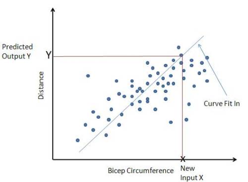
Suppose you have a habit of collecting weird datasets and you end up collecting up a dataset that gives the circumference of biceps of many men and the distance a javelin is thrown by each of them. And you want to predict for an unknown individual, given the circumference of his biceps how far can he throw the javelin.

Ofcourse there would be a number of reasons that would affect the distance a javelin would go, such as skill (which is essentially non-quantitative?), height, the kid of footwear worn, run-up distance, state of health etc. These would be the some of the many features that would affect that end result (distance a javelin is thrown). What I essentially mean is that the circumference of the biceps isn’t a realistic feature to predict how far a javelin can be thrown. But let’s assume that there is only one feature and it can make reasonable predictions. This over-simplification is only made so that the process can be visualized in a graph.

Suppose you collect about 80 such examples (which you call the training examples) and plot your data as such:

Now the problem given to you is: Given you have the bicep-circumference measurement of an unknown individual, predict how far he can throw the javelin.

How would one do it?

What we would do is to fit in some curve in the above training set (the above plot). And when we have to make a prediction we simply plug in that value in our curve and find the corresponding value for the distance. Something illustrated below.

The curve can be represented in a number of ways. However, if the curve was to be represented linearly (that’s why it’s called linear regression) it could be written as :

Where is the hypothesis, and  are unknown parameters which are to be learnt from the data and is the input feature. It is noteworthy that this is like the slope intercept form of the line.

In the above, for simplicity I considered only one feature, there could be many more. In the more general case:

The ‘s are called the parameters (to be learnt from the data) that will decide the nature of the curve.

We see that the equation involves features of the training examples (‘s), therefore using this, the task of the learning algorithm will be to decide the most optimum values of using the training set. This can be easily done by something like Gradient Descent.

For any new example, we’d have the features and parameters would already be known by running gradient descent using the training set. We simply have to plug in the value of in equation to get a prediction.

To sum up : Like I mentioned, we use the training set to fit in a optimal curve and then try to predict unseen inputs by simply plugging in its values to the “equation of the curve”.

Now, it goes without saying that we could fit in a “simple” model to the training set or a more “complex” model. A simple model would be linear say something like:

and a complex model could be something like this:

.

It’s to be noted that in the above the same feature is used in different ways, the second model uses to create more features such as , and so on. Clearly the second representation is more complex than the first as it will exploit more patterns in the data (it has more parameters).

However this increase in complexity can lead to problems, in the same way if the model is too simple it can lead to problems. This is illustrated below:

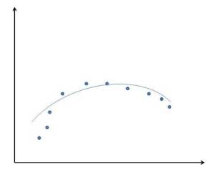
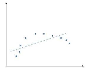
[Fig 1 (Left) and Fig 2 (Right)]

The figure on the left has a “simple model” fit into the training set. Clearly there are patterns in the data that the model would never take into account, no matter how big the training set goes. Paraphrasing this in more concrete terms, it’s clear that the relationship between and is not linear. So if we try to fit in a linear model to it, not matter how much we train it, there would always be some patterns in the data that the model would fail to subsume.

What this means is, what is learnt from the training set will not be generalised well to unknown examples (this is because, it might be that the unknown example comes from that part of the distribution that the model fails to account for and thus the prediction for it would be very inaccurate).

The figure on the right has a “complex” model fit into the same set, clearly the model fits the data very well. But again it is not a good predictor as it does not represent the general nature of the spread of the data but rather takes into account the idiosyncrasies of the same. This model would make very good predictions on the data from the training set itself, but it would not generalize well to unknown examples.

A more appropriate fit would be something like this :

Now we can move to a definition of the generalization error, The generalization error of a hypothesis is its expected error on examples that are not from the training set. For an example on understanding generalization refer to the part labeled “Van-Gogh Chagall and Pigeons” in this post.

The models shown in figures 1 and 2 have HIGH generalization errors. However each suffer from entirely different problems.

______

Bias : Like already mentioned : In the model shown in fig. 1, no matter how much the model is trained, There would always be some patterns in the data that the model would fail to capture. This is because the model has a high BIAS. Bias of a model is the expected generalization error even if we were to fit in a very large training-set.

Thus the linear model shown in figure 1 suffers from high bias and will underfit the data.

Variance : Apart from bias there is another component that has a bearing on the generalization error. That is the variance of the model fit into the training set.

This is shown in fig. 2. We see that even though that the model fits in very well in the training set, there is the risk that we are fitting patterns that are idiosyncratic to the training examples and may not represent the general pattern between and .

Since we might be fitting spurious patters and exaggerating minor fluctuations in the data, such a model would still give a high generalization error and will over-fit the data. In such a case we say that the model has a high variance.

The Trade-off : When deciding on a model to fit onto the training set, there is a trade-off between the bias and the variance. If either is high that would mean the generalizing ability of the model would be low (generalization error would be high). In other words, if the model is too simple i.e if it has too few parameters it would have a high bias and if the model is too complex it would have a high variance. While deciding on a model we have to strike a balance between the two.

A very famous example that illustrates this trade-off goes like this:

[Suppose there is an exacting biologist who studies and classifies green trees in detail. He would be the example of an over-trained or over-fit model and would declare if he sees a tree with non-green leaves like above that it is not a tree at all]

[An under-trained or under-fit model would be like the above biologist’s lazy brother, who on seeing a cucumber which is green declares that it is a tree]

Both of the above have poor generalization. We wish to select a model that has an appropriate trade-off between the two.

______

So why do we need Learning Theory?

Learning theory is an interesting subject in its own right. It, however also hones our intuitions on how to apply learning algorithms properly  giving us a set of rules of the thumb that guide us on how to apply learning algorithms well.

Learning theory can answer quite a few questions :

1. In the previous section there was a small discussion on bias and variance and the trade-off between the two. The discussion sounds logical, however there is no meaning to it unless it is formalized. Learning theory can formalize the bias variance trade-off. This helps as we can then make a choice on choosing the model with just the right bias and variance.

2. Learning Theory leads to model selection methods by which we can choose automatically what model would be appropriate for a certain training set.

3. In Machine Learning, models are fit on the training set. So what we essentially get is the training error. But what we really care about is the generalization ability of the model or the ability to give good predictions on unseen data.

Learning Theory relates the training error on the training set and the generalization error and it would tell us how doing well on the training set might help us get better generalization.

4. Learning Theory actually proves conditions in which the learning algorithms will actually work well. It proves bounds on the worst case performance of models giving us an idea when the algorithm would work properly and when it won’t.

The next post would answer some of the above questions.

______

Onionesque Reality Home >>

Read Full Post »

Taught Bio-Informatics (UG)

I am in the process of winding up taking a basic course on Bio-Informatics, it is offered as an elective subject for final year under-graduate Information Technology students.  I preferred taking this course as a visiting faculty on weekends as managing time in the week is hard (though i did take some classes on weekdays).

______

[Gene Clustering : (a) shows clusters (b) uses hierarchical clustering (c) uses k-means (d)  SOM finds clusters which are arranged in grids. Source : Nature Biotechnology 23, 1499 – 1501 (2005) by Patrick D’haeseleer]

Why Bio-Informatics?

The course (out of the ones offered in Fall) I would have preferred taking the most would have been a course on AI. There is no course on Machine Learning or Pattern Recognition at the UG level here, and the course on AI comes closest as it has sufficient weight given to Neural Nets and Bayesian Learning.

The only subject that comes nearest to my choice as AI was not available, was Bio-Informatics as about 60 percent of the syllabus was Machine Learning, Data Mining and Pattern Recognition. And it being a basic course gave me the liberty to take these parts in much more detail as compared to the other parts. And that’s exactly why taking up Bio-Informatics even though it’s not directly my area was not a bad bargain!

______

The Joys of Teaching:

This is the first time that I have formally taken a complete course, I have taken work-shops and given talks quite a few times before. But never taken a complete course.

I have always enjoyed teaching. When I say I enjoy teaching, I don’t necessarily mean something academic. I like discussing ideas in general

If I try to put down why I enjoy teaching, there might be some reasons:

• There is an obvious inherent joy in teaching that few activities have for me. When i say teaching here, like I said before I don’t just mean to talk about formal teaching, but rather the more general meaning of the term.

• It’s said that there is no better way to learn than to teach. Actually that was the single largest motivation that prompted me to take that offer.

• Teaching gives me a high! The time I get to discuss what I like (and teach), I forget things that might be pressing me at other times of the day. I tend to become a space-cadet when into teaching. It’s such a wonderful experience!

• One more reason that i think i like teaching is this : I have a wide range of reading (or atleast am interested in) and I have noticed that the best way it gets connected and in most unexpected ways is in discussions. You don’t get people who would be interested in involved discussions very often, also being an introvert means the problem is further compounded. Teaching gives me a platform to engage in such discussions. Some of the best ideas that I have got, borrowing from a number of almost unrelated areas is while discussing/teaching. And this course gave me a number of ideas that I would do something about if I get the chance and the resources.

• Teaching also gives you the limits of your own reading and can inspire you to plug the deficiencies in your knowledge.

• Other than that, I take teaching or explaining things as a challenge. I enjoy it when I find out that I can explain pion exchanges to friends who have not seen a science book after grade 10. Teaching is a challenge well worth taking for a number of reasons!

From this specific course the most rewarding moment was when a couple of groups approached me after the conclusion of classes to help them a little with their projects. Since their projects are of moderate difficulty and from pattern recognition, I did take that up as a compliment for sure! Though I can not say I can “help” them,  I don’t like using that word, it sounds pretentious, I would definitely like to work with them on their projects and hopefully would learn something new about the area.

______

Course:

I wouldn’t be putting up my notes for the course, but the topics I covered included:

1. Introduction to Bio-Informatics, Historical Overview, Applications, Major Databases, Data Management, Analysis and Molecular Biology.

2. Sequence Visualization, structure visualization, user interface, animation verses simulation, general purpose technologies, statistical concepts, microarrays, imperfect data, quantitative randomness, data analysis, tool selection, statistics of alignment, clustering and classification, regression analysis.

3. Data Mining Methods & Technology overview, infrastructure, pattern recognition & discovery, machine learning methods, text mining & tools, dot matrix analysis, substitution metrics, dynamic programming, word methods, Bayesian methods, multiple sequence alignment, tools for pattern matching.

4. Introduction, working with FASTA, working with BLAST, filtering and capped BLAST, FASTA & BLAST algorithms & comparison.

Like I said earlier, my focus was on dynamic programming, clustering, regression (linear, locally weighted), Logistic regression, support vector machines, Neural Nets, an overview of Bayesian Learning. And then introduced all the other aspects as applications subsequently and covered the necessary theory then!

______

Resources:

All my notes for the course were hand-made and not on , so it would be impossible to put them up now (they were basically made from a number of books and the MIT-OCW).

H0wever I would update this space soon enough linking to all the resources I would recommend.

______

I am looking forward to taking a course on Digital Image Processing and Labs the next semester, which begins December onwards (again as a visiting instructor)! Since Image Processing is closer to the area I am interested in deeply (Applied Machine Learning – Computer Vision), I am already very excited about the possibility!

______

Onionesque Reality Home >>

Read Full Post »