Face Recognition/Authentication Using Support Vector Machines

This post is part of a series on face recognition, I have been posting on face recognition for a while. There would be at least 7-8 more posts in the near future on the topic. Though I can not promise a time frame within which all would be up.

Previous Related Posts:

1. Face Recognition using Eigenfaces and Distance Classifiers – A Tutorial

2. Face Recognition in Bees

3. A Huge Collection of Datasets (Post links to a number of face image databases)

4. Why are Support Vector Machines called so?

This post would reference two of my posts. One on SVMs and the other on Face Recognition using Eigenfaces.

Note: This post focuses on the idea behind using SVMs for face recognition and authentication. In future posts I will cover the various packages that can be used to implement SVMs and how to go about using them, and specifically for face recognition. The same can be easily extended to other similar problems such as content based retrieval systems, speech recognition, character or signature verification systems as well.

_____

Difference between Face Authentication (Verification) and Face Recognition (also called identification):

This might seem like a silly thing to start with. But for the sake of completeness, It is a good point to start with.

Face Authentication can be considered a subset of face recognition. Though due to the small difference there are a few non-concurrent parts in both the systems.

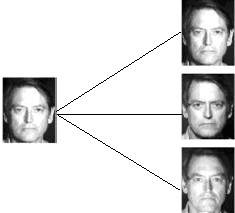
Face Authentication (also called verification) involves a one to one check that compares an input image (also called a query image, probe image or simply probe) with only the image (or class) that the user claims to be. In simple words, if you stand in front of a face authentication system and claim to be a certain user, the system will ONLY check if you are that user or not.

Face Recognition (or Identification) is another thing, though ofcourse related. It involves a one to many comparison of the input image (or probe or query image) with a template library. In simple words, in a face recognition system the input image will be compared with ALL the classes and then a decision will be made so as to identify to WHO the the input image belongs to. Or if it does not belong to the database at all.

Like I just said before, though both Authentication and Recognition are related there are some differences in the method involved, which are obvious due to the different nature of both.

_____

A Touch-Up of Support Vector Machines:

A few posts ago I wrote a post on why Support Vector Machines had this rather “seemingly” un-intuitive name. It had a brief introduction to SVMs as well. For those completely new to Support Vector Machines this post should help. I’ll still add a little for this post.

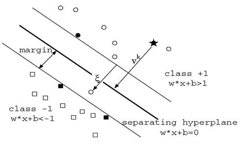
Support Vector Machine is a binary classification method that finds the optimal linear decision surface between two classes. The decision surface is nothing but a weighted combination of the support vectors. In other words, the support vectors decide the nature of the boundary between the two classes. Take a look at the image below:

The SVM takes in labeled training examples , where represents the features and the class label, that could be either 1 or -1.  On training we obtain a set of Support Vectors , multipliers , and the term . To understand what does, look at the above figure. It is somewhat like the intercept term in the equation of a straight line, . The terms and determine the orientation of the hyperplane while determines the actual position of the hyperplane.

As is indicated in the diagram, the linear decision surface is :

where

where are the support vectors.

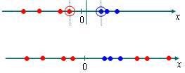
The above holds when the data (classes) is linearly separable. Sometimes however, that’s not the case. Take the following example:

The two classes are indicated by the two different colors. The data is clearly not LINEARLY separable.

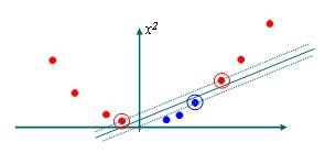
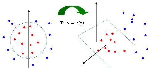
However when mapped onto two dimensions, a linear decision surface between them can be made with ease.

Take another example. In this example the data is not linearly separable in 2-D, so they are mapped onto three dimensions where a linear decision surface between the classes can be made.

By Cover’s Theorem it is more likely that a data-set not linearly separable in some dimension would be linearly separable  in a higher dimension. The above two examples are simple, sometimes the data might be linearly separable at very high dimensions, maybe at infinite dimensions.

But how do we realize it? This done by employing the beautiful Kernel Trick. In place of the inner products we use a suitable Mercer Kernel. I don’t believe it is a good idea to discuss kernels here, or it will be a needless digression from face recognition. I promise to discuss it some time later.

Thus the non-linear decision surface changes from to:

Where represents a Kernel. It could be a Radial Basis (Gaussian) Kernel, A linear Kernel, A polynomial Kernel or a custom Kernel. :)

_____

Face Authentication is a two class problem. As I have mentioned earlier, here the system is presented with a claimed identity and it has to make a decision whether the claimant is really that person or not. The SVM in such applications will have to be fed with the images of one person, which will constitute one class and the other class will consist of images of other people other than that person. The SVM will then generate a linear decision surface.

For a input/probe image , the identity is accepted if:

Or it is rejected. We can parameterize the decision surface by modifying the above as:

Then, a claim will be accepted if for a probe,

_____

Now face recognition is a class problem. Where is the number of classes (or individuals).  Whereas the traditional Support Vector Machine is a binary classifier. So we’ll make a few changes to the way we are representing the faces to suit our classifier. I will come back to this in a while.

Feature Extraction: The faces will have to be represented by some appropriate features, these could be weights obtained using the Eigenfaces method, or using gabor features or anything else. I have written a post earlier that talked of a face recognition system based on Eigenfaces. I would direct the reader to check face representation using Eigenfaces there.

Using Eigenfaces, each probe could be represented as a vector of weights:

After obtaining such a weight vector for the input or probe image and for all the other images stored in the library, we were simply finding the Euclidean or the Mahalanobis distance of the weight vector of the probe image with those of the images in the template library.  And then were recognizing the probe as a face that gave the minimum score provided it was below a certain threshold. I have discussed this is much detail there. And since I have, I would not discuss this again here.

_____

Representation in Difference Space:

SVMs are binary classifiers, that is – they give the class which might be 1 or -1, so we would have to modify the representation of faces a little bit than what we were doing in that previous post to make it somewhat more desirable. In the previous approach that is “a view based or face space approach”, each image was encoded separately. Here, we would change the representation and encode faces into a difference space. The difference space takes into account the dissimilarities between faces.

In the difference space there can be two different classes.

1. The class that encodes the dissimilarities between different images of the same person,

2. The other class encodes the dissimilarities between images of other people. These two classes are then given to a SVM which then generates a decision surface.

As  I wrote earlier, Face recognition traditionally can be thought of as a class problem and face authentication can be thought of as a instances two class problem. To reduce it to a two class problem we formulate the problem into a difference space as I have already mentioned.

Now consider a training set having training images belonging to individuals. Each individual can have more than one image, that means ofcourse. It is from that we generate the two classes I mentioned above.

1. The within class differences set. This set takes into account the differences in the images of the same class or individual. In more formal terms:

Where and are images and indicates that they belong to the same person.

This set contains the differences not just for one individual but for all individuals.

2. The between class differences set. This set gives the dissimilarities of different images of different individually. In more formal terms:

Where and are images and indicates that they do not belong to the same person.

_____

Face Authentication:

For Authentication the incoming probe and a claimed identity is presented.

Using this, we first find out the similarity score:

We then accept this claim if it lies below a certain threshold or else reject it. I have discussed the need for a threshold at the end of this post, please have a look. is to be found heuristically.

_____

Face Recognition:

Consider a set of images , and a probe which is to be indentified.

We take and score it with every image in the set :

The image with the lowest score but below a threshold is recognized. I have written at the end of this post explaining why this threshold is important. This threshold is mostly chose heuristically.

_____

References and Important Papers

1. Face Recognition Using Eigenfaces, Matthew A. Turk and Alex P. Pentland, MIT Vision and Modeling Lab, CVPR ‘91.

2. Eigenfaces Versus Fischerfaces : Recognition using Class Specific Linear Projection, Belhumeur, Hespanha, Kreigman, PAMI ‘97.

3. Eigenfaces for Recognition, Matthew A. Turk and Alex P. Pentland, Journal of Cognitive Neuroscience ‘91.

4. Support Vector Machines Applied to Face Recognition, P. J. Phillips, Neural Information Processing Systems ’99.

5. The Nature of Statistical Learning Theory (Book), Vladimir Vapnik, Springer ’99.

6. A Tutorial on Support Vector Machines for Pattern Recognition, Christopher J. C. Burges, Data Mining and Knowledge Discovery, ’99

_____

Onionesque Reality Home >>

Read Full Post »

Zero Crossings as an Effective Feature In Speech Recognition for Embedded Applications

Motivation: About a couple of months back i was wondering on designing a speaker dependent speech recognizer on the 8051 micro-controller or any of its derivatives for simple machine control. We would of course need an isolated word (or digit) recognizer.

Problem: Speech recognizers can be implemented using Hidden Markov Models or Artificial Neural Networks. There are plenty of such systems in place. However the problem with these algorithms is that they are computationally pretty intensive, and thus can not be implemented on a simple 8 bit fixed point micro-processor, and that is what we need for simple machine control applications. So there is a need for a simpler algorithm.

All these algorithms also employ a short term feature vector to take care of the non-stationary nature of speech. Generally the vector length is so chosen that the nature of the signal in this band is quasi-stationary. Feature vectors are an area of active research. Generally however at the university level, Mel Frequency Cepstrum Coefficients (MFCC) or Linear Predictive Coefficients are taken as features. These too require computations that are beyond the scope of a simple processor/ micro controller like the 8051.

Solution: I was thinking what could be done to reduce this burden and choose a simpler feature so that it could be implemented on 8051. While researching on this i came across a paper[1]. This papers deals with this problem exactly!

The researchers have used only zero crossings of the speech signal to determine the feature vector. Since this novel feature extraction method is based on zero crossings only, it just needs a one bit A to D conversion[2]. This feature extraction is computationally very simple and does not require the speech signal to be pre-processed.

This feature vector is basically the histogram of the time interval between successive zero-crossings of the utterance in a short time window[1]. These feature vectors for each window are then combined together to form a feature matrix. Since we are dealing with only small time series (isolated words), we can employ Dynamic Time Warping to compare the input matrix with the reference matrix’ stored. I will discuss this in another post sometime.

To obtain this vector the following steps need to be followed.

1. The speech signal x(t) is band-pass filtered to give s(t).

2. s(t) is then subjected to infinite amplitude clipping with the help of a ZCD to give u(t).

3. u(t) is then sampled at say 8Khz to give u[n]. The feature extraction is carried out on u[n].

4. u[n] is divided in a number of short time windows for every one of the calculated W samples.

5. The histogram for each of this short time window is found. The histogram(or vector) is found as follows: The number of times ONLY ONE sample is recorded between successive zero crossings will constitute the element number 1 of the vector. The number of times ONLY TWO samples are recorded between successive zero crossings will constitute the element number two of the feature vector and so on. In this way we construct an histogram which is an appropriate feature vector.

These vectors then can be combined for all windows to get the feature matrix. These as i said earlier can be compared using DTW/DDTW/Fast DTW or some other algorithm.

As an example take an utterance for the number three in Hindi which is spoken as “teen”. The first plot below gives the waveform for the utterance. The second plot gives the end-point detected version of the same, end point detection reduces computations (and hence the memory required) by removing the “useless” portions of the utterance which do not contain any intelligence.

The surface plot for the above utterance by me for the matrix (where, as i have mentioned implicitly the rows represent the windows and the columns represent the histogram terms) prepared is as:

References:

[1] A Microprocessor based Speech Recognizer for Isolated Hindi Digits, Ashutosh Saxena and Abhishek Singh, IEEE ACE.

[2] Zero-Crossing-Based Linear Prediction for Speech Recognition, Lipovac, Electronics Letters, pages 90-92, vol. 25 Issue 2,19 Jan 1989.

Onionesque Reality Home >>

Read Full Post »

The Working of a Bird Swarm

This post is following the previous post in which i mentioned about the rules governing the motion of a bird swarm.

The video below is a breathtaking, sublime, amazing recording of thousands of starlings in a flock before roosting. This is from the UK country-side. While it is another awesome demonstration of how the “imagination” of nature can be like, it also gives a perfect example of how the entire swarm is organized and how it moves. Modern researchers are trying to imitate such emergent behavior to use in fields like robotics, data mining, internet mathematics, optimization etc etc.

How do birds exactly do this?

Here is an excerpt from a talk that i had given at a technical event in October ’07.

In a swarm if we say that there are ‘N’ number of agents, then we can say that these autonomous agents are in a way co-operating to achieve a global objective. This global objective can be better foraging, constructing shelter, serving as a defence mechanism among others. This apparent collective intelligence emerges from very simple individual agents. The actions of these agents are governed by local rules and through the interactions of the N agents the swarm achieves a global objective. A kind of “self organization” emerges in these systems. We see that there is no central controller in such cases. Swarm intelligence gives a basis which makes it possible to explore collective (or distributed) problem solving without centralized control or without the provision of a global model. ^[1]

The individual (but autonomous) agent does not follow directives from a central authority or work according to some global plan. As a common example, a bird in a flock, only adjusts its movements to coordinate with the movements of its flock mates or more precisely the members that are its neighbors. It simply tries to stay close to its neighbors, but avoid collisions with them. Each bird does not take commands from any leader bird since there is no lead bird. Any bird can fly anywhere in the swarm, either in the middle or the front or the back of the swarm. Swarm behavior gives the birds some distinct advantages like protection from predators, and searching for food (effectively in a swarm each bird is exploiting the eyes of every other bird). Scientists are trying to find out how these birds, fish etc move in flocks, schools in a way that appears orchestrated. A school of fish and a flock of birds move as if all the “steps” were pre planned. For one moment they are moving towards the left and in another they are darting towards the right. Among these researchers in 1987, Reynolds created a boidor bird-oid (bird like) model. This is a distributed behavioral model, to simulate the motion of a flock of birds on a computer ^[2]. Each boid is implemented as an agent which moves according to its own understanding of the dynamic environment. A boid observes the following rules. First, is that a boid must move away from boids that are too close, so as to reduce the chance of collisions. Second, boid must fly in the general direction that the flock is moving. Third, a boid should minimize exposure to the flock’s exterior by moving toward the perceived center of the flock. Flake later ^[3] added a Fourth rule, a boid should move laterally away from any boid that blocks its view. This boid model seems reasonable if we consider it from another point of view, that of it acting according to attraction and repulsion between neighbors in a flock. The repulsion relationship results in the avoidance of collisions and attraction makes the flock keep shape, i.e., copying movements of neighbors can be seen as a kind of attraction.

This is what i was talking about in the previous post. A certain set of rules is followed that would give a certain shape to the swarm, if the set is altered so will be the shape and maybe functionality as well!

Sounds nice, now how can these simple rules be modeled on a computer? They can be done using NetLogo. Here is a sample model . To get a good idea about the intricacies adjust the population, the turn angles and the vision. For playing around with the model and making your own you are instructed to go through the writeup to this model on the above page.

References:

[1] E. Bonabeau, M. Dorigo, and G. Theraulaz, Swarm Intelligence: From Natural to Artifcial Systems. NY: Oxford Univ. Press, 1999.

[2] C. Reynolds, ‘Flocks, herds, and schools: A distributed behavioral model,” Comp. Graph, vol. 21, no. 4, pp. 25{34, 1987.

[3] G. Flake, The Computational Beauty of Nature. Cambridge, MA: MIT Press, 1999.

Read Full Post »

Morphogenesis and Swarm Robotics

Here is an amazing video!

Something about this video first from the you-tube information about it.

An introduction to swarm intelligence, swarm robotics and morphogenesis. This video won the Best Video award at the AAAI-07 conference Vancouver Canada. The scientific research was performed by Anders Lyhne Christsensen, Rehan O’Grady and Marco Dorigo. The video was directed by Andreia Onofre.

Swarm Intelligence is an AI technique that is based on the collective behavior of decentralised and self organised systems. Take an ant colony for example, an ant hill is an extremely complex structure, with even things like temperature control in place. It is difficult to imagine a simple ant doing any of it! So it is basically the “swarm” of ants that is responsible for such emergent and intelligent solutions though the “constituents” of the systems (i.e ants) are simple and independent “units”. Like ants also can pick up prey many times their weight by forming very precise structures encircling the object under consideration.

like in the picture below the ants take up a comparatively much heavier fly.

photo credit with full regards : here>>

The video basically explains the same and also gives an idea on how it could be done using robots. For example a bird swarm can make very different and complex shapes depending on the set of rules under use (which in turn will depend on the scenario). I will accompany this statement by a post on a bird swarm and how they do it sometime soon. If you change the set of rules you could change the shape you get, and most of these shapes could be used to perform some intelligent task. This gives the swarm a lot of flexibility. This is basically what is Morphogenesis.

Morphogenesis could be used by a swarm of robots to move heavy objects (as an illustration to this have a look at this video, in which a group of robots pull away a child. The video can be seen here>>) which could be used in fire-fighting applications etc, to bridge gaps etc. A swarm of nano-bots could use morphogenesis to perform very specific tasks inside the human body!

Please have a look at this award winning video!

I personally thank and congratulate the director of this video for putting it all so succinctly in a matter of under 5 minutes.

Read Full Post »