A short note on how the Graph Laplacian is a natural analogue of the Laplacian in vector analysis.
For a twice differentiable function  on the euclidean space, the Laplacian of ,
  is the div(grad()) or the divergence of the gradient of . Let’s consider the laplacian in two dimensions:

To get an intuition about what it does, it is useful to consider a finite difference approximation to the above:

The above makes it clear that the Laplacian behaves like a local averaging operator. Infact the above finite difference approximation is used in image processing (say, when h is set to one pixel) to detect sharp changes such as edges, as the above is close to zero in smooth image regions.
____________________________
The finite difference approximation intuitively suggests that a discrete laplace operator should be natural. At the same time, the Graph Theory literature defines the Graph Laplacian as the matrix  (where
  is the degree matrix and
  the adjacency matrix of the graph
  , both are defined below). It is not obvious that this matrix
  follows from the div(grad(f)) definition mentioned above. The purpose of this note is to explicate in short on how this is natural, once the notion of gradient and divergence operators have been defined over a graph.
First of all the two most natural matrices that can be associated with a graph are defined below:
____________________________
There are two natural matrices that are used to specify a simple graph  with vertex set
 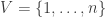 and edge set
  : The Adjacency matrix and the Incidence matrix
  .
.
The Adjacency matrix is defined as a  matrix such that:
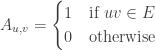
To define the  incidence matrix , we need to fix an orientation of the edges (for our purpose an arbitrary orientation suffices), then:
Now suppose we have a real valued function over  ,
,  . For , we view this as a column vector indexed by the vertices.
Similarly let  be a real valued function over the edges
  ,
,  (again, we view this as a row vector indexed by the edges).
Now, consider the following map:  (which is now a vector indexed by ). The value of this map at any edge
  is simply the difference of the values of at the two end points of the edge
  i.e.
i.e.  . This makes it somewhat intuitive that the matrix is some sort of a difference operator on . Given this “difference operator” or “discrete differential” view,
  can then be viewed as the gradient that measures the change of the function along the edges of . Thus the map is just the gradient operator.
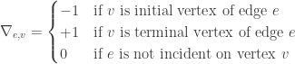
Like the above, now we consider the following map:  (which is now a vector indexed by ). Recall that was defined on the edges. The value of this map at any vertex
  is
is  . If we were to view as describing some kind of a flow on the edges, then is the net outbound flow on the vertex
  , which is just the divergence. Thus the map
  is just the divergence operator.
Now consider  (note that this makes sense since
  is a column vector), going by the above, this should be the divergence of the gradient. Thus, the analogy with the “real” Laplacian makes sense and the matrix
  is appropriately called the Graph Laplacian.
Using the definition of , a simple computation yields the following for  :
:
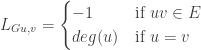
Looking at the above and recalling the definition for the adjacency matrix , it is easy to see that  , where is the diagonal matrix with
  . This is just the familiar definition that I mentioned at the start.
PS: From the above it is also clear that the Laplacian is positive semidefinite. Indeed, consider  , which is written as
Read Full Post »


