An informal summary of a recent project I had some involvement in.
Motivation: Why care about Metric Learning?
In many machine learning algorithms, such as k-means, Support Vector Machines, k-Nearest Neighbour based classification, kernel regression, methods based on Gaussian Processes etc etc – there is a fundamental reliance, that is to be able to measure dissimilarity between two examples. Usually this is done by using the Euclidean distance between points (i.e. points that are closer in this sense are considered more similar), which is usually suboptimal in the sense that will be explained below. Being able to compare examples and decide if they are similar or dissimilar or return a measure of similarity is one of the most fundamental problems in machine learning. Ofcourse a related question is: What does mean by “similar” afterall?
To illustrate the above let us work with k-Nearest Neighbour classification. Before starting, let us just illustrate the really simple idea (of kNN classification) by an example: Consider the following points in  , with the classes marked by different colours.
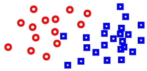
Now suppose we have a new point – marked with black – whose class is unknown. We assign it a class by looking at the nearest neighbors and taking the majority vote:

Some notes on kNN:
A brief digression first before moving on the problem in the above (what is nearest?). kNN classifiers are very simple and yet in many cases they can give excellent performance. For example, consider the performance on the MNIST dataset, it is clear that kNN can give competitive performance as compared to other more complicated models.
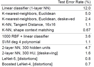
Moreover, they are simple to implement, use local information and hence are inherently nonlinear. The biggest advantage in my opinion is that it is easy to add new classes (since no retraining from scratch is required) and since we average across points, kNN is also relatively robust to label noise. It also has some attractive theoretical properties: for example kNN is universally consistent (as the number of points approaches infinity, with appropriate choice of k, the kNN error will approach the Bayes Risk).
Notion of “Nearest”:
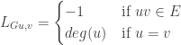
At the same time, kNN classifiers also have their disadvantages. One is related to the notion of “nearest” (which falls back on what was talked about at the start) i.e. how does one decide what points are “nearest”. Usually such points are decided on the basis of the Euclidean distance on the native feature space which usually has shortfalls. Why? Because nearness in the Euclidean space may not correspond to nearness in the label space i.e. points that might be far off in the Euclidean space may have similar labels. In such cases, clearly the notion of “near” using the euclidean distance is suboptimal. This is illustrated by a set of figures below (adapted from slides by Kilian Weinberger):
An Illustration:
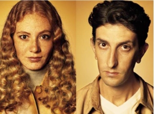
Consider the image of this lady – now how do we decide what is more similar to it?
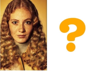
Someone might mean similar on the basis of the gender:
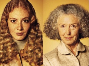 Or on the basis of age:
Or on the basis of the hairstyle!
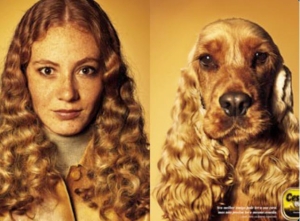
Similarity depends on the context! Something that the euclidean distance in the native feature space would fail to capture. This context is provided by labels.
Distance Metric Learning:
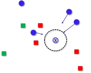
The goal of Metric Learning is to learn a distance metric, so that the above label information is incorporated in the notion of distance i.e. points that are semantically similar are now closer in the new space. The idea is to take the original or native feature space, use the label information and then amplify directions that are more informative and squish directions that are not. This is illustrated in this figure – notice that the point marked in black would be incorrectly classified in the native feature space, however under the learnt metric it would be correctly classified.

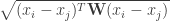
It is worthwhile to have a brief look at what this means. The Euclidean distance (with  ) is defined by
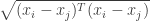
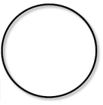
as also was evident in the above figure, this corresponds to the following euclidean ball in 2-D
A family of distance measure may be defined using an inner product matrix. These are called the Mahalanobis metrics.
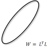
The learnt metric affects a rescaling and rotation of the original space. The goal is now to learn this  using the label information so that the new distances correspond better to the semantic context. It is easy to see that when , the above is still a distance metric.
Learning  :
:
Usually the real motivation for metric learning is to optimize for the kNN objective i.e. learn the matrix  so that the kNN error is reduced. But note that directly optimizing for the kNN loss is intractable because of the combinatorial nature of the optimization (we’ll see this in a bit), so instead, is learnt as follows:
1. Define a set of “good” neighbors for each point. The definition of “good” is usually some combination of proximity to the query point and label agreement between the points.
2. Define a set of “bad” neighbours for each point. This might be a set of points that are “close” to the query point but disagree on the label (i.e. inspite of being close to the query point they might give a wrong classification if they were chosen to classify the query point).
3. Set up the optimization problem for such that for each query point, “good” neighbours are pulled closer to it while “bad” neighbours are pushed farther away, and thus learn so as to minimize the leave one out kNN error.
The exact formulation of “good” and “bad” varies from method to method. Here are some examples:
In one of the earliest papers on distance metric learning by Xing, Ng, Jordan and Russell (2002) – good neighbors are similarly labeled k points. The optimization is done so that each class is mapped into a ball of fixed radius. However no separation is enforced between the classes. This is illustrated in the following figure (the query point is marked with an X, similarly labeled k points are moved into a ball of a fixed radius):
One problem with the above is that the kNN objective does not really require that similarly labeled points are clustered together, hence in a way it optimizes for a harder objective. This is remedied by the LMNN described briefly below.
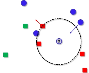
One of the more famous Metric Learning papers is the Large Margin Nearest Neighbors by Weinberger and Saul (2006). Here good neighbors are similarly labeled k points (and the circle around x is the distance of the farthest of the good neighbours) and “worst offenders” or “bad” neighbours are points that are of a different class but still in the nearest neighbors of the query point. The optimization is basically a semidefinite program that works to pull the good neighbours towards the query point and a margin is enforced by pushing the offending points out of this circle. Thus in a way, the goal in LMNN is to deform the metric in such a way that the neighbourhood for each point is “pure.

There are many approaches to the metric learning problem, however a few more notable ones are:
1. Neighbourhood Components Analysis (Goldberger, Roweis, Hinton and Salakhutdinov, 2004): Here the piecewise constant error of the kNN rule is replaced by a soft version. This leads to a non-convex objective that can be optimized by gradient descent. Basically, NCA tries to optimize for the choice of neighbour at the price of losing convexity.
2. Collapsing Classes (Globerson and Roweis, 2006): This method attempts to remedy the non-convexity above by optimizing a similar stochastic rule while attempting to collapse each class to one point, making the problem convex.
3. Metric Learning to Rank (McFee and Lankriet, 2010): This paper takes a different take on metric learning, treating it as a ranking problem. Note that given a fixed p.s.d matrix a query point induces a permutation on the training set (in order of increasing distance). The idea thus is to optimize the metric for some ranking measure (such as precision@k). But note that this is not necessarily the same as requiring correct classification.
Neighbourhood Gerrymandering:
As a motivation we can look at the cartoon above for LMNN. Since we are looking to optimize for the kNN objective, the requirement to learn the metric should just be correct classification. Thus, we should need to push the points to ensure the same. Thus we can have the circle around x as simply the distance of the farthest point in the k nearest neighbours (irrespective of class). Now, we would like to deform the metric such that enough points are pulled in and pushed out of this circle so as to ensure correct classification. This is illustrated below.
This method is akin to the common practice of Gerrymandering, in drawing up borders of election districts so as to provide advantages to desired political parties. This is done by concentrating voters from a particular party and/or by spreading out voters from other parties. In the above, the “districts” are cells in the Voronoi diagram defined by the Mahalanobis metric and “parties” are class labels voted for by each neighbour.
Motivations and Intuition:
Now we can step back a little from the survey above, and think a bit about the kNN problem in somewhat more precise terms so that the above approach can be motivated better.
For kNN, given a query point and a fixed metric, there is an implicit latent variable: The choice of the k “neighbours”.
Given this latent variable – inference of the label for the query point is trivial – since it is just the majority vote. But notice that for any given query point, there can exist a very large number of choices of k points that may correspond to correct classification (basically any set of points with majority of correct class will work). Now we basically want to learn a metric so that we prefer one of these sets over any set of k neighbours which would vote for a wrong class. In particular, from the sets that affects correct classification we would like to pick the set that is on average most similar to the query point.
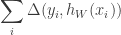
We can write kNN prediction as an inference problem with a structured latent variable being the choice of k neighbours.
The learning then corresponds to minimizing a sum of structured latent hinge loss and a regularizer. Computing the latent hinge loss involves loss-augmented inference – which is basically looking for the worst offending k points (points that have high average similarity with the query point, yet correspond to a high loss). Given the combinatorial nature of the problem, efficient inference and loss-augmented inference is key. Optimization can basically be just gradient descent on the surrograte loss. To make this a bit more clear, the setup is described below:
Problem Setup:
Suppose we are given  training examples that are represented by a “native” feature map,
  with with class labels
 ![\mathbf{y} = [y_1, \dots, y_N]^T](https://s0.wp.com/latex.php?latex=%5Cmathbf%7By%7D+%3D+%5By_1%2C+%5Cdots%2C+y_N%5D%5ET&bg=ffffff&fg=333333&s=0&c=20201002) with
with ![y_i \in [\mathbf{R}]](https://s0.wp.com/latex.php?latex=y_i+%5Cin+%5B%5Cmathbf%7BR%7D%5D&bg=ffffff&fg=333333&s=0&c=20201002) , where
, where ![[\mathbf{R}]](https://s0.wp.com/latex.php?latex=%5B%5Cmathbf%7BR%7D%5D&bg=ffffff&fg=333333&s=0&c=20201002) stands for the set
stands for the set  .
.
Suppose are also provided with a loss matrix  with
with  being the loss incurred by predicting
  when the correct class is
  . We assume that
  and
and  .
.
Now let  be a set of examples in
  .
.
As stated earlier, we are interested in the Mahalanobis metrics:

For a fixed  we may define the distance of
  with respect to a point
  as:
as:
Therefore, the set of k-Nearest Neighbours of in is:

For any set of  examples from we can predict the label of by a simple majority vote.

The kNN classifier therefore predicts  .
.
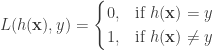
Thus, the classification loss incurred using the set can be defined as:
Learning and Inference:
One might want to learn so as to minimize the training loss:
However as mentioned in passing above, this fails because of the intractable nature of the classification loss  . Thus we’d have to resort to the usual remedy: define a tractable surrograte loss.
It must be stressed again that the output of prediction is a structured object  . The loss in structured prediction penalizes the gap between score of the correct structured output and the score of the “worst offending” incorrect output. This leads to the following definition of the surrogate:
![L(x,y,W) = \max_h [S_W(x,h) + \Delta(y,h)] - \max_{h: \Delta(y,h) = 0} S_W(x,h)](https://s0.wp.com/latex.php?latex=L%28x%2Cy%2CW%29+%3D+%5Cmax_h+%5BS_W%28x%2Ch%29+%2B+%5CDelta%28y%2Ch%29%5D+-+%5Cmax_%7Bh%3A+%5CDelta%28y%2Ch%29+%3D+0%7D+S_W%28x%2Ch%29&bg=ffffff&fg=333333&s=0&c=20201002)
This corresponds to our earlier intuition on wanting to learn such that the gap between the “good neighbours” and “worst offenders” is increased.
So, although the loss above was arrived at by intuitive arguments, it turns out that our problem is an instance of a familiar type of problem: Latent Structured Prediction and hence the machinery for optimization there can be used here as well. The objective for us corresponds to:
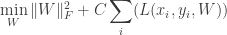
Where  is the Frobenius norm.
Note that the regularizer is convex, but the loss is not convex to the subtraction of the max term i.e. now it is a difference of convex functions which means the concave convex procedure may be used for optimization (although we just use stochastic gradient descent). Also note that the optimization at each step needs an efficient subroutine to determine the correct structured output (inference of the best set of neighbours) and the worst offending incorrect structured output (loss augmented inference i.e. finding the worst set of neighbors). Turns out that for this problem this is possible (although not presented here).
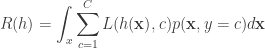
It is interesting to think about how this approach extends to regression and to see how it works when the embeddings learnt are not linear.


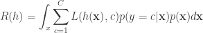
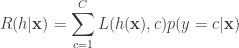
![R(h) = \mathbb{E}_{\mathbf{x},y} [L(h(\mathbf{x}),y)]](https://s0.wp.com/latex.php?latex=R%28h%29%C2%A0+%3D+%5Cmathbb%7BE%7D_%7B%5Cmathbf%7Bx%7D%2Cy%7D+%5BL%28h%28%5Cmathbf%7Bx%7D%29%2Cy%29%5D&bg=ffffff&fg=333333&s=0&c=20201002)


 on the euclidean space, the Laplacian of
  is the div(grad(

 (where
  is the degree matrix and
  the adjacency matrix of the graph
  , both are defined below). It is not obvious that this matrix
  follows from the div(grad(f)) definition mentioned above. The purpose of this note is to explicate in short on how this is natural, once the notion of gradient and divergence operators have been defined over a graph.
 with vertex set
  and edge set
  : The Adjacency matrix
  .
. matrix such that:
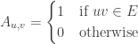
 incidence matrix
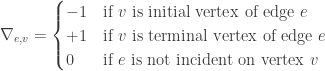
 ,
,  . For
. For  be a real valued function over the edges
  ,
,  (again, we view this as a row vector indexed by the edges).
 (which is now a vector indexed by
  is simply the difference of the values of
  i.e.
i.e.  . This makes it somewhat intuitive that the matrix
  can then be viewed as the gradient that measures the change of the function
  (which is now a vector indexed by
  is
is 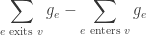 . If we were to view
  , which is just the divergence. Thus the map
  is just the divergence operator.
 (note that this makes sense since
  is a column vector), going by the above, this should be the divergence of the gradient. Thus, the analogy with the “real” Laplacian makes sense and the matrix
  is appropriately called the Graph Laplacian.
 :
:
 , where
  . This is just the familiar definition that I mentioned at the start.
 , which is written as


 . The idea was to estimate at each training point, the gradient of this unknown function
  where
where  is the number of classes (let us say for the purpose of this discussion, that for each data point we have a probability distribution over the classes, a
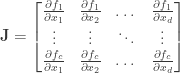
 ![\displaystyle \Bigg[ \frac{\partial f}{\partial x_1}, \frac{\partial f}{\partial x_2}, \dots, \frac{\partial f}{\partial x_d} \Bigg]](https://s0.wp.com/latex.php?latex=%5Cdisplaystyle+%5CBigg%5B+%5Cfrac%7B%5Cpartial+f%7D%7B%5Cpartial+x_1%7D%2C+%5Cfrac%7B%5Cpartial+f%7D%7B%5Cpartial+x_2%7D%2C+%5Cdots%2C+%5Cfrac%7B%5Cpartial+f%7D%7B%5Cpartial+x_d%7D+%5CBigg%5D&bg=ffffff&fg=333333&s=0&c=20201002)
 may be estimated in a similar manner as estimating gradients as in the previous posts. Which leads us to define the quantity
 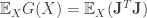 .
. defined in the previous post is simply the quantity for the special case when
  is a symmetric and positive semi-definite matrix, which defines a smoothly varying inner product in the tangent space
  , for each point
  and
and  . This associated p.s.d matrix is called the metric tensor. In the above case, since
 is a specific metric (more general metrics are dealt with in areas such as metric learning).
 and otherwise?
 for some unknown smooth
  is
is  dimensional
 may be written as
  where
where  .
.  projects down the data to only
  . It is important to note that
  is given by
 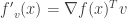 or
or  .
. .
. , the gradient outer product matrix
  be the eigenvectors of
 sample points, gives a sample gradient outer product. There is some work that shows that some of these estimators are
  , where
  .
.


