Over the past 4-5 months whenever there is some time to spare, I have been working through The Cauchy-Schwarz Master Class by J. Michael Steele. And, although I am still left with the last two chapters, I have been reflecting on the material already covered in order to get a better perspective on what I have been slowly learning over the months. This blog post is a small exercise in this direction.
Ofcourse, there is nothing mysterious about proving the Cauchy-Schwarz inequality; it is fairly obvious and basic. But I thought it still might be instructive (mostly to myself) to reproduce some proofs that I know out of memory (following a maxim of my supervisor on a white/blackboard blogpost). Although, why Cauchy-Schwarz keeps appearing all the time and what makes it so useful and fundamental is indeed quite interesting and non-obvious. And like Gil Kalai notes, it is also unclear why is it that it is Cauchy-Schwarz which is mainly useful. I feel that Steele’s book has made me appreciate this importance somewhat more (compared to 4-5 months ago) by drawing to many concepts that link back to Cauchy-Schwarz.
Before getting to the post, a word on the book: This book is perhaps amongst the best mathematics book that I have seen in many years. True to its name, it is indeed a Master Class and also truly addictive. I could not put aside the book completely once I had picked it up and eventually decided to go all the way. Like most great books, the way it is organized makes it “very natural” to rediscover many susbtantial results (some of them named) appearing much later by yourself, provided you happen to just ask the right questions. The emphasis on problem solving makes sure you make very good friends with some of the most interesting inequalities. The number of inequalities featured is also extensive. It starts off with the inequalities dealing with “natural” notions such as monotonicity and positivity and later moves onto somewhat less natural notions such as convexity. I can’t recommend this book enough!
Now getting to the proofs: Some of these proofs appear in Steele’s book, mostly as either challenge problems or as exercises. All of them were solvable after some hints.
________________
Proof 1: A Self-Generalizing proof
This proof is essentially due to Titu Andreescu and Bogdan Enescu and has now grown to be my favourite Cauchy-Schwarz proof.
We start with the trivial identity (for 
Identity 1:

Expanding we have
Rearranging this we get:

Further: 
Rearranging this we get the following trivial Lemma:
Lemma 1:
Notice that this Lemma is self generalizing in the following sense. Suppose we replace 


But we can apply Lemma 1 to the second term of the right hand side one more time. So we would get the following inequality:

Using the same principle 

Now substitute 


This is just the Cauchy-Schwarz Inequality, thus completing the proof.
________________
Proof 2: By Induction
Again, the Cauchy-Schwarz Inequality is the following: for

For proof of the inequality by induction, the most important thing is starting with the right base case. Clearly 


To prove the base case, we simply expand the expressions. To get:

Which is just:

Or:

Which proves the base case.
Moving ahead, we assume the following inequality to be true:

To establish Cauchy-Schwarz, we have to demonstrate, assuming the above, that

So, we start from 
we further have,

Now, we can apply the case for

Thus, using this in the R. H. S of 

Or,

This proves the case 
________________
Proof 3: For Infinite Sequences using the Normalization Trick:
We start with the following question.
Problem: For 


Note that this is easy to establish. We simply start with the trivial identity 

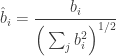
Next, take 

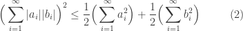
From this it immediately follows that
Now let


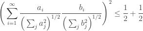
Which simply gives back Cauchy’s inequality for infinite sequences thus completing the proof:

________________
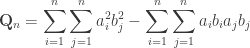
Proof 4: Using Lagrange’s Identity
We first start with a polynomial which we denote by 

The question to now ask, is 
Next, as J. Michael Steele puts, we pursue symmetry and rewrite the above so as to make it apparent.
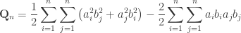
Thus, we now have:

This makes it clear that

Now, reversing the step we took at the onset to write the L.H.S better, we simply have:
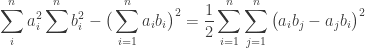
This is called Lagrange’s Identity. Now since the R.H.S. is always greater than or equal to zero. We get the following inequality as a corrollary:

This is just the Cauchy-Schwarz inequality, completing the proof.
________________
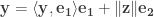
Proof 5: Gram-Schmidt Process gives an automatic proof of Cauchy-Schwarz
First we quickly review the Gram-Schmidt Process: Given a set of linearly independent elements of a real or complex inner product space 


for 
Keeping the above in mind, assume that 


Giving: 


Now note that: 


Which is just the Cauchy-Schwarz inequality when 
________________
Proof 6: Proof of the Continuous version for d =2; Schwarz’s Proof
For this case, the inequality may be stated as:
Suppose we have 


The proof given by Schwarz as is reported in Steele’s book (and indeed in standard textbooks) is based on the following observation:
The real polynomial below is always non-negative:


________________
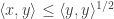
Proof 7: Proof using the Projection formula
Problem: Consider any point 


If 


This is fairly elementary to establish. To find the value of 


which is simply:


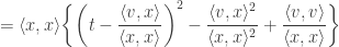

So, the value of 
Therefore, the minimum squared distance is given by the expression below:

Note that the L. H. S is always positive. Therefore we have:

Rearranging, we have:

Which is just Cauchy-Schwarz, thus proving the inequality.
________________
Proof 8: Proof using an identity
A variant of this proof is amongst the most common Cauchy-Schwarz proofs that are given in textbooks. Also, this is related to proof (6) above. However, it still has some value in its own right. While also giving an useful expression for the “defect” for Cauchy-Schwarz like the Lagrange Identity above.
We start with the following polynomial:


To find the minimum of this polynomial we find its derivative w.r.t

Clearly we have 


Just rearrangine and simplifying:

This proves Cauchy-Schwarz inequality.
Now suppose we are interested in an expression for the defect in Cauchy-Schwarz i.e. the difference 


i.e. Defect =
Which is just:

This defect term is much in the spirit of the defect term that we saw in Lagrange’s identity above, and it is instructive to compare them.
________________
Proof 9: Proof using the AM-GM inequality
Let us first recall the AM-GM inequality:
For non-negative reals 
![\displaystyle \sqrt[n]{x_1 x_2 \dots x_n} \leq \Big(\frac{x_1 + x_2 + \dots x_n}{n}\Big)](https://s0.wp.com/latex.php?latex=%5Cdisplaystyle+%5Csqrt%5Bn%5D%7Bx_1+x_2+%5Cdots+x_n%7D+%5Cleq+%5CBig%28%5Cfrac%7Bx_1+%2B+x_2+%2B+%5Cdots+x_n%7D%7Bn%7D%5CBig%29&bg=ffffff&fg=333333&s=0&c=20201002)
Now let us define 

Now consider the trivial bound (which gives us the AM-GM): 


Using the above, we have:

Summing over

But note that the L.H.S equals 1, therefore:


Writing out 


Thus proving the Cauchy-Schwarz inequality.
________________
Proof 10: Using Jensen’s Inequality
We begin by recalling Jensen’s Inequality:
Suppose that ![f: [p, q] \to \mathbb{R}](https://s0.wp.com/latex.php?latex=f%3A+%5Bp%2C+q%5D+%5Cto+%5Cmathbb%7BR%7D&bg=ffffff&fg=333333&s=0&c=20201002)


![x_i \in [p, q]](https://s0.wp.com/latex.php?latex=x_i+%5Cin+%5Bp%2C+q%5D+&bg=ffffff&fg=333333&s=0&c=20201002)

Now we know that 

Now, for 


Which gives:
Rearranging this just gives the familiar form of Cauchy-Schwarz at once:

________________
Proof 11: Pictorial Proof for d = 2
Here (page 4) is an attractive pictorial proof by means of tilings for the case 
________________


 […] by this formula Galileo converted a natural law inherent in the actual motion of bodies into an a priori constructed mathematical function, and that is what physics endeavors to accomplish for every phenomenon […]. This law is much better design than our tax laws. It has been designed by nature, who seems to lay her plans with a fine sense for simplicity and harmony. But then nature is not, as our income and excess profits tax laws are, hemmed in having to be comprehensible to our legislators and chambers of commerce. […]”

 by the intersection of
  hyperplanes?
 case.
case. , then the maximum number of possible regions is obviously two.

 i.e. 4 hyerplanes, this number is 11 as shown below:
 be an arrangement of


