Recently, in course of a project that I had some involvement in, I came across an interesting quadratic form. It is called in the literature as the Gradient Outer Product. This operator, which has applications in supervised dimensionality reduction, inverse regression and metric learning can be motivated in two (related) ways, but before doing so, the following is the set up:
Setup: Suppose we have the usual set up as for nonparametric regression and (binary) classification i.e. let  for some unknown smooth
  , the input
  is
is  dimensional
1. Supervised Dimensionality Reduction: It is often the case that varies most along only some relevant coordinates. This is the main motivation behind variable selection.
The idea in variable selection is the following: That  may be written as
  where
where  .
.  projects down the data to only
  relevant coordinates (i.e. some features are selected by while others are discarded).
This idea is generalized in Multi-Index Regression, where the goal is to recover a subspace most relevant to prediction. That is, now suppose the data varies significantly along all coordinates but it still depends on some subspace of smaller dimensionality. This might be achieved by letting from the above to be  . It is important to note that is not any subspace, but rather the -dimensional subspace to which if the data is projected, the regression error would be the least. This idea might be further generalized by means of mapping to some non-linearly, but for now we only stick to the relevant subspace.
How can we recover such a subspace?
________________
2. Average Variation of : Another way to motivate this quantity is the following: Suppose we want to find the direction in which varies the most on average, or the direction in which varies the second fastest on average and so on. Or more generally, given any direction, we want to find the variation of along it. How can we recover these?
________________
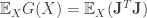
The Expected Gradient Outer Product: The expected gradient outer product of the unknown classification or regression function is the quantity: 
The expected gradient outer product recovers the average variation of in all directions. This can be seen as follows: The directional derivative at  along
along  is given by
 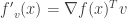 or
or  .
.
From the above it follows that if does not vary along  then must be in the null space of
  .
.
Infact it is not hard to show that the relevant subspace as defined earlier can also be recovered from . This fact is given in the following lemma.
Lemma: Under the assumed model i.e.  , the gradient outer product matrix is of rank at most . Let
 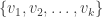 be the eigenvectors of corresponding to the top eigenvalues of . Then the following is true:

This means that a spectral decomposition of recovers the relevant subspace. Also note that the Gradient Outer Product corresponds to a kind of a supervised version of Principal Component Analysis.
________________
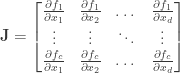
Estimation: Ofcourse in real settings the function is unknown and we are only given points sampled from it. There are various estimators for , which usually involve estimation of the derivatives. In one of them the idea is to estimate, at each point a linear approximation to . The slope of this approximation approximates the gradient at that point. Repeating this at the  sample points, gives a sample gradient outer product. There is some work that shows that some of these estimators are statistically consistent.
________________
Related: Gradient Based Diffusion Maps: The gradient outer product can not isolate local information or geometry and its spectral decomposition, as seen above, gives only a linear embedding. One way to obtain a non-linear dimensionality reduction would be to borrow from and extend the idea of diffusion maps, which are well established tools in semi supervised learning. The central quantity of interest for diffusion maps is the graph laplacian  , where
  is the degree matrix and
  the adjacency matrix of the nearest neighbor graph constructed on the data points. The non linear embedding is obtained by a spectral decomposition of the operator
  or its powers
  .
.
As above, a similar diffusion operator may be constructed by using local gradient information. One such possible operator could be:

Note that the first term is the same that is used in unsupervised dimension reduction techniques such as laplacian eigenmaps and diffusion maps. The second term can be interpreted as a diffusion on function values. This operator gives a way for non linear supervised dimension reduction using gradient information.
The above operator was defined here, however no consistency results for the same are provided.
Also see: The Jacobian Inner Product.
________________
Read Full Post »


![\displaystyle \Bigg[ \frac{\partial f}{\partial x_1}, \frac{\partial f}{\partial x_2}, \dots, \frac{\partial f}{\partial x_d} \Bigg]](https://s0.wp.com/latex.php?latex=%5Cdisplaystyle+%5CBigg%5B+%5Cfrac%7B%5Cpartial+f%7D%7B%5Cpartial+x_1%7D%2C+%5Cfrac%7B%5Cpartial+f%7D%7B%5Cpartial+x_2%7D%2C+%5Cdots%2C+%5Cfrac%7B%5Cpartial+f%7D%7B%5Cpartial+x_d%7D+%5CBigg%5D&bg=ffffff&fg=333333&s=0&c=20201002)